


1. Introduction
Signal modulation is an important technique in wireless communication. It has important application value in military field, signal monitoring, etc. Automatic Modulation Recognition (AMR), as a major part of signal modulation, has the core task of distinguishing the modulation mode used in modulated signals and estimating the modulation-related parameters without relevant a priori information. With the development of wireless communication technology and the complexity of the signal environment, the recognition accuracy of traditional modulation recognition methods is limited under different signal-to-noise ratio conditions, and the application of Deep Learning (DL) to AMR has gradually become mainstream.
In this paper, we propose an automatic modulation recognition method based on a hybrid CNN-Transformer model. Convolutional Neural Network (CNN) is responsible for extracting local time-frequency features of the signal, reducing the dimensionality of the data and improving the model's ability to perceive the short-time information. Transformer uses the self-attention mechanism to model the global temporal dependence of the signal and enhance the recognition ability of complex modulation patterns. In this study, simulation experiments are conducted based on the DeepSig RadioML 2018.01A public dataset to test the classification performance of the model under different signal-to-noise ratios, and the CNN-Transformer combination model proposed in this paper can show better recognition ability under high signal-to-noise ratio conditions, which can provide an efficient and robust solution for automatic modulation recognition, and maintain a high level of recognition performance under complex channel environments.
2. Signal modulation and Deep Learning
2.1. Signal modulation basics
2.1.1. Signal modulation principles and applications
Signal modulation is the process or processing method of changing certain characteristics (such as amplitude, frequency, or phase) of one waveform according to another waveform or signal [1]. In the communication system, the main purpose of the modulation technique is to guarantee the effective transmission of the signal in the channel, and to provide a solid basic support for the subsequent data demodulation and processing as well. The form of signal modulation can be divided into analog modulation and digital modulation according to the type of the original signal. Common forms of digital signal modulation include amplitude keying (ASK), frequency shift keying (FSK), phase shift keying (PSK) and quadrature amplitude modulation (QAM). In practical applications, modulation identification technology is widely used in electronic reconnaissance, spectrum detection and many other military and civilian fields.
2.1.2. Development of signal modulation techniques
Early research was mostly based on instantaneous and statistical features for classification, and the classifiers used by engineers included Support Vector Machines (SVMs) as well as Decision Trees, etc. In 2016, as deep learning continued to make technical breakthroughs, the success of techniques such as residual neural networks in image processing inspired researchers to introduce deep learning into signal processing [2]. Subsequent research aimed at improving the accuracy of modulation mode recognition, mainly focusing on the attempt of new networks and the combination between different networks to realize the diversity of modulation recognition modes.
2.2. Application of Deep Learning in signal processing
2.2.1. Basics of Deep Learning
Deep Learning (DL) is a branch of machine learning and is an algorithm that uses neural networks as an architecture to learn representations of information.
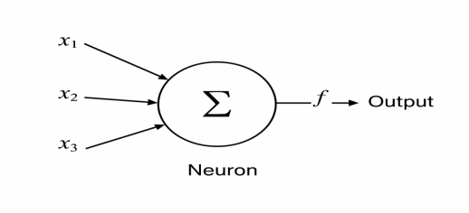
Among them, neural network is a computational model inspired by the traditional biological nervous system and consists of a large number of artificial neurons as shown in Figure 1. It is able to learn patterns and features from a large amount of data by adjusting the weights of different parameters to achieve complex mapping relationships [3]. Compared with traditional methods, deep learning has the advantage of using more efficient feature extraction algorithms instead of acquiring features manually, reducing the dependence on domain knowledge and improving the generalization ability of the model.
2.2.2. Convolutional neural networks in a nutshell
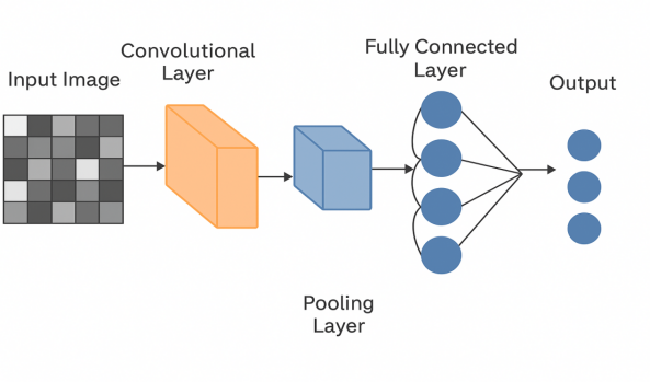
CNN, or Convolutional Neural Network, is a special neural network model designed based on biological visual processing.CNN uses at least one layer of convolutional operation in the network architecture instead of matrix multiplication in traditional networks, and is able to effectively extract the local features of the input data by means of local connectivity and weight sharing. Its main components include a convolutional layer, a pooling layer and a fully connected layer [4]. As shown in Figure 2 the convolutional layer extracts features through convolutional operations, the pooling layer is used for dimensionality reduction and to improve the robustness of the model, and the fully connected layer is used to output the classification results. Nowadays, with the continuous development of deep learning, CNNs are widely used in Computer Vision (CV) [5]. In signal processing tasks, CNNs can extract local features from raw signals, but have limited ability to model long time dependencies or global information.
2.2.3. Transformer in a nutshell
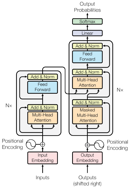
Transformer is a deep learning model based on a self-attention mechanism proposed by Google Brain in 2017. It was initially applied in the field of Natural Language Processing (NLP), but has been widely used in CV in recent years. As shown in Figure 3, the transformer consists of two modules, Encoder and Decoder. The encoder part is mainly used to extract global feature information from the input sequence. The Decoder is similar in structure to the Encoder, but with the addition of Masked Multi-Head Attention, which prevents the model from obtaining subsequent information in advance of the current output. Unlike traditional neural networks, the transformer is able to process sequential data in parallel, which is suitable for long time series modeling [6]. Compared to traditional CNNs that focus more on local features, transformer is better at modeling the signal as a whole. It shows good recognition efficiency and accuracy in signal modulation recognition tasks.
3. Deep Learning based automatic modulation recognition experiments
3.1. Experimental data analysis
3.1.1. Data set description
|
Dataset |
Modulation Types |
Modulation List |
Samples |
Dimension |
SNR |
|
RML2018.01a |
24 types |
OOK, 4ASK, 8ASK, BPSK, QPSK, 8PSK, 16PSK, 32PSK, 16APSK, 32APSK, 64APSK, 128APSK, 16QAM, 32QAM, 64QAM, 128QAM, 256QAM, AM-SSB-WC, AM-SSB-SC, AM-DSB-WC, AM-DSB-SC, FM, GMSK, OQPSK |
2,555,904 |
[2,1024] |
-20:2:30 |
In this study, the DeepSig RadioML 2018.01A dataset is used, and the data are stored as In-phase and Quadrature (IQ) in the format of a floating-point type 2D vector, with the dimension of a single sample being 1024 sampling points, each of which contains information about both I/Q channels. The labels are stored in One-Hot coded form and are subsequently converted to integer category indexes.AS shown in Table 1. The dataset covers 24 modulation modes with 4096 data entries for each modulation mode, totaling 2555904 data entries. These modulations cover common signal types in analog and digital communications, including analog modulation versus digital modulation, and the signals are uniformly distributed over 26 SNR levels ranging from -20 dB to 30 dB.
3.1.2. Preprocessing of the dataset
In the processing of the original dataset, each SNR=10db was used as a criterion for slicing, and each modulation data under different intervals was extracted to form a set of six samples. At the same time, each selected SNR interval is sliced twice and divided into training set, test set A and validation set B in the ratio of 6:2:2, and saved as independent HDF5 files. Random indexing is used to ensure a balanced distribution of samples during the partitioning process. Each file contains three sets of data: X (IQ signal), Y (modulation label) and Z (SNR label).
3.2. Network architecture and training program
3.2.1. Cnn-transformer model architecture design
In order to extract the multilevel features of the modulated signal more effectively, a hybrid model combining CNN and Transformer is designed and adopted in this study. As shown in Figure 4, this model combines the advantages of both: CNN is more suitable for extracting the local time-domain features of the modulated signal, whereas the Transformer is better at modeling the global context and long-term dependencies of the signal. information and long time dependencies of the signal. Through this combination of local and global feature extraction mechanisms, the model is able to understand the structure of the modulated signal more comprehensively.
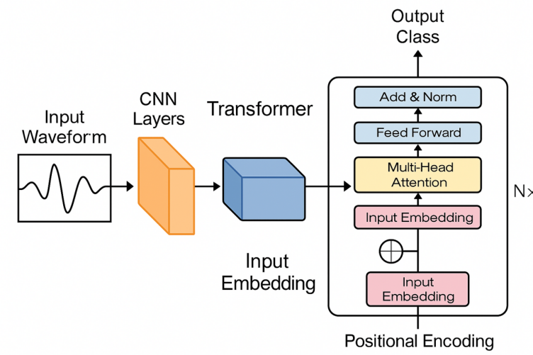
The input to the model is a one-dimensional IQ signal sequence with a size of 1024 × 2, which means that there are 1024 time points for each sample, and each time point contains both real and imaginary part information. The input data is first passed through a three-layer 1D convolutional network with a convolutional kernel size of 3, a same filling mode, and a number of channels of 32, 64, and 128. After each layer of convolution, a ReLU activation function is accessed to enhance the nonlinear expression ability of the model. After the convolution operation, the model is able to extract local temporal features such as waveform inflection points, abrupt trends and frequency changes.
This process can be briefly represented by the following pseudo-code:
# Input: x, shape [Batch, 2, 1024]
# - Batch: Number of input samples
# - 2: I/Q channels (In-phase and Quadrature)
# - 1024: Time steps for each sample
# First convolution layer with 32 filters
x = Conv1D(in_channels=2, out_channels=32, kernel_size=3, padding=1)(x)
x = ReLU()(x) # Non-linear activation to introduce non-linearity
# Second convolution layer with 64 filters
x = Conv1D(32, 64, kernel_size=3, padding=1)(x)
x = ReLU()(x)
# Third convolution layer with 128 filters
x = Conv1D(64, 128, kernel_size=3, padding=1)(x)
x = ReLU()(x)
# Output shape after convolution: [Batch, 128, 1024]
# - 128 channels for enriched feature representation
# - 1024 time steps preserved
Next, the convolutional output is dimensioned to match the input format of the Transformer encoder. Learnable positional coding is then added to preserve temporal information. The Transformer encoder consists of three layers of encoders, each containing a multi-head attention module with a feedforward neural network module, with the hidden size set to 128, the feedforward dimensionality to 256, and the number of attention heads to 4. With this stacked structure, the model is able to extract long-range correlation features layer-by-layer. The model is able to extract long-distance correlation features layer by layer through this stacked structure.
The Transformer coding process can be simplified as shown in the following pseudo-code:
# Input: x, shape [Batch, 1024, 128]
# - 1024: Time steps (sequence length)
# - 128: Feature dimension from CNN
# Step 1: Add positional encoding to preserve temporal order
x = x + PositionalEncoding()
# Step 2: Multi-head attention layers for global dependency modeling
for _ in range(3):
# TransformerEncoderLayer consists of:
# - Multi-Head Attention: Attends to different parts of the sequence
# - Feedforward Network: Enhances feature representation
x = TransformerEncoderLayer(embed_dim=128, num_heads=4, ff_dim=256)(x)
# Output shape: [Batch, 1024, 128]
# - Time steps and feature dimensions remain consistent
The model performs mean pooling of the Transformer's output along the time dimension to form a fixed-length vector, which is then classified by the fully-connected layer, and ultimately outputs 24 classes of modulation mode predictions.
# Input: x, shape [Batch, 1024, 128]
# - 1024: Time steps
# - 128: Feature dimension
# Step 1: Global Average Pooling to compress time dimension
# This reduces the time sequence [1024] to a single feature vector [128]
x = MeanPooling(dim=1)(x) # shape becomes [Batch, 128]
# Step 2: Fully connected layer to classify 24 modulation types
output = Linear(128, 24)(x) # shape becomes [Batch, 24]
# The output is the probability distribution over 24 classes
3.2.2. Model training and optimization strategies
In order to ensure that the model has good generalization ability and robustness under different signal-to-noise ratio environments, this paper carries out careful design and optimization of the model training process. In the training process, the classification loss function based on cross entropy (CrossEntropyLoss) is used, and the optimizer is chosen to be AdamW, which has a good performance in deep learning, and the optimizer combines the weight decay mechanism, which can help to prevent the model from overfitting. In terms of specific settings, the batch size is set to 64 during training, the initial learning rate is 5e-5, and the ReduceLROnPlateau learning rate scheduling strategy is introduced. When the validation set loss does not decrease significantly in several rounds of training, the learning rate will be automatically reduced, thus helping the model to jump out of the local optimum. Meanwhile, in order to enhance the robustness of the model to channel perturbations with different modulation sample variations, two data enhancement strategies are introduced into the training data: one is to flip the IQ data with 10% probability, and the other is to superimpose a small Gaussian noise with 10% probability, so as to improve the model's fault-tolerance in complex environments. In addition, a gradient trimming operation is introduced in the training to prevent gradient explosion, and the Early Stopping strategy is activated when there is no boost in loss to terminate the training to avoid overfitting. The main flow of the training process can be briefly represented as follows:
# Training configuration
batch_size = 64
learning_rate = 5e-5
num_epochs = 100
# Initialize optimizer and loss function
optimizer = AdamW(model.parameters(), lr=learning_rate)
criterion = CrossEntropyLoss()
# Training loop
for epoch in range(num_epochs):
for x_batch, y_batch in train_loader:
# === Data Augmentation ===
if rand() < 0.1:
x_batch = flip(x_batch) # 10% chance to flip
if rand() < 0.1:
x_batch += torch.randn_like(x_batch) * 0.01 # Add Gaussian noise
# === Forward Propagation ===
preds = model(x_batch)
loss = criterion(preds, y_batch)
# === Backpropagation and Optimization ===
optimizer.zero_grad()
loss.backward()
optimizer.step()
# Learning rate scheduler
scheduler.step(loss)
# Early Stopping if no improvement
if early_stop_triggered():
break
Through the above optimization and control strategies, the model not only performs stably on the training set, but also shows strong adaptive ability on the test set, which lays a good foundation for the analysis of the subsequent experimental results.
3.3. Experimental results and analysis
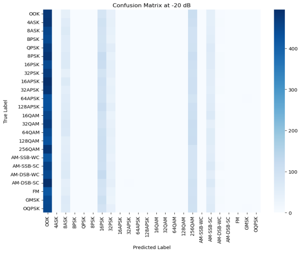
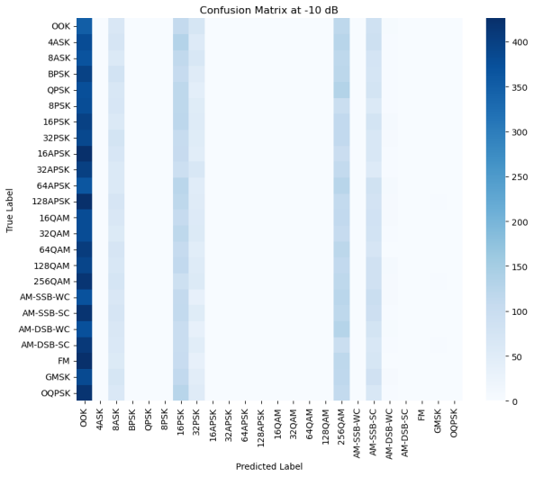

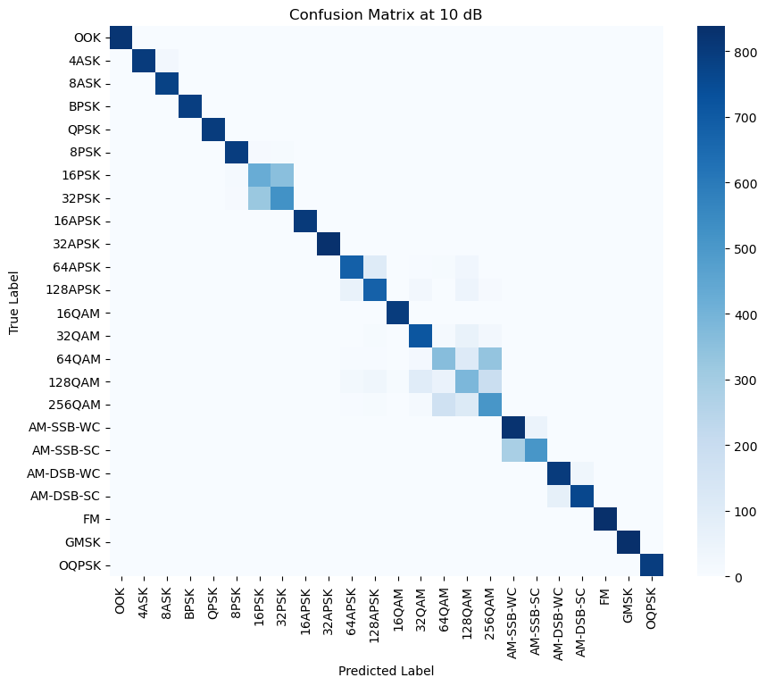

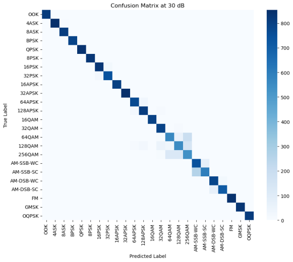
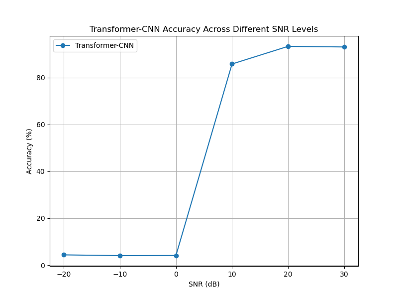
Figure 5: (a) Confusion matrix at -20db (b) Confusion matrix at -10db (c) Confusion matrix at 0db (d) Confusion matrix at 10db (e) Confusion matrix at 20db (f) Confusion matrix at 30db (g)Transformer-CNN Accuracy Across Different SNR Levels
In order to verify the recognition ability of the model under different SNRs, this paper conducted tests under six SNR intervals from -20 dB to 30 dB. As shown in Figure 5, the overall recognition accuracy of the model increases significantly as the SNR increases. At low SNRs such as -20 dB and -10 dB, the confusion between modulation types is more serious, especially in the OOK and APSK categories where the misrecognition rate is higher. However, above 10 dB, the accuracy rate improves significantly, indicating that the model's ability to distinguish modulation types is significantly enhanced. By observing the confusion matrix, it can be found that some modulation types still have subtle confusion even under high SNR conditions, such as 64QAM and 128QAM, which may be due to the similarity between the two waveforms under specific channel characteristics. In addition, some modulations (e.g., FM, AM-SSB-SC) show high accuracy at all SNRs, indicating that the model has good stability in feature extraction for such signals. As can be seen from the accuracy plot, the model accuracy shows an upward trend with increasing SNR, breaking through 85% at 10 dB and stabilizing above 90% in the 20 dB and 30 dB intervals, which indicates that the designed CNN-Transformer model has an excellent modulation recognition capability in high SNR.
4. Conclusion
In this paper, we mainly proposed and implemented a deep learning model based on the fusion of CNN and Transformer, and tested its performance in the automatic modulation recognition task. Experiments show that the fusion model has an average recognition accuracy of up to 90% in high SNR environments (above 10db), but lower in low SNR environments. Through the confusion matrix analysis under different SNR conditions, it is found that there is still confusion between some modulation modes, and the discriminative ability of the model can be further optimized in the future. There are still some shortcomings in this study, such as the basic network model has not been introduced for comparison experiments. In addition, the current model does not involve cutting-edge training strategies such as self-supervised learning and migration learning. Future research directions include optimizing model compression techniques for deployment in resource-constrained environments, exploring few-shot learning to improve recognition with limited training data, and extending the model to real-world multi-path fading environments.
References
[1]. M. Li, "Research on Automatic Modulation Recognition Technology of Digital Communication Signals, " Master's thesis, Harbin Engineering University, Harbin, China, 2012.
[2]. Q. A. Qiknow, "Automatic Modulation Recognition Based on Transformer (RML2018), " CSDN Blog, Aug. 2024. Available: https: //blog.csdn.net/QAQIknow/article/details/144815416.
[3]. I. Kang, "Automatic Modulation Recognition Based on Deep Learning, " CSDN Blog, Aug. 2018. Available: https: //blog.csdn.net/illikang/article/details/82019945.
[4]. C. Chen, N. Zhang, C. Yang, Y. Gao and Y. Sheng, "Multiple-Stream Model with CNN-LSTM for Automatic Modulation Recognition, " 2023 International Conference on Microwave and Millimeter Wave Technology (ICMMT), Qingdao, China, 2023, pp. 1-3, doi: 10.1109/ICMMT58241.2023.10277458.
[5]. S. Lin, Y. Zeng, and Y. Gong, "Learning of Time-Frequency Attention Mechanism for Automatic Modulation Recognition, " arXiv preprint arXiv: 2111.03258, 2021.
[6]. Ashish Vaswani, Noam Shazeer, Niki Parmar, Jakob Uszkoreit, Llion Jones, Aidan N. Gomez, Łukasz Kaiser, and Illia Polosukhin. 2017. Attention is all you need. In Proceedings of the 31st International Conference on Neural Information Processing Systems (NIPS'17). Curran Associates Inc., Red Hook, NY, USA, 6000–6010.
[7]. R. Zhang, "Deep Learning-Based Automatic Modulation Recognition with Code, " CSDN Blog, Aug. 6, 2022. Available: https: //blog.csdn.net/qq_40935157/article/details/126190599
Cite this article
Yu,M. (2025). Application of Deep Learning to Automatic Modulation Recognition. Applied and Computational Engineering,175,18-29.
Data availability
The datasets used and/or analyzed during the current study will be available from the authors upon reasonable request.
Disclaimer/Publisher's Note
The statements, opinions and data contained in all publications are solely those of the individual author(s) and contributor(s) and not of EWA Publishing and/or the editor(s). EWA Publishing and/or the editor(s) disclaim responsibility for any injury to people or property resulting from any ideas, methods, instructions or products referred to in the content.
About volume
Volume title: Proceedings of CONF-CDS 2025 Symposium: Application of Machine Learning in Engineering
© 2024 by the author(s). Licensee EWA Publishing, Oxford, UK. This article is an open access article distributed under the terms and
conditions of the Creative Commons Attribution (CC BY) license. Authors who
publish this series agree to the following terms:
1. Authors retain copyright and grant the series right of first publication with the work simultaneously licensed under a Creative Commons
Attribution License that allows others to share the work with an acknowledgment of the work's authorship and initial publication in this
series.
2. Authors are able to enter into separate, additional contractual arrangements for the non-exclusive distribution of the series's published
version of the work (e.g., post it to an institutional repository or publish it in a book), with an acknowledgment of its initial
publication in this series.
3. Authors are permitted and encouraged to post their work online (e.g., in institutional repositories or on their website) prior to and
during the submission process, as it can lead to productive exchanges, as well as earlier and greater citation of published work (See
Open access policy for details).
References
[1]. M. Li, "Research on Automatic Modulation Recognition Technology of Digital Communication Signals, " Master's thesis, Harbin Engineering University, Harbin, China, 2012.
[2]. Q. A. Qiknow, "Automatic Modulation Recognition Based on Transformer (RML2018), " CSDN Blog, Aug. 2024. Available: https: //blog.csdn.net/QAQIknow/article/details/144815416.
[3]. I. Kang, "Automatic Modulation Recognition Based on Deep Learning, " CSDN Blog, Aug. 2018. Available: https: //blog.csdn.net/illikang/article/details/82019945.
[4]. C. Chen, N. Zhang, C. Yang, Y. Gao and Y. Sheng, "Multiple-Stream Model with CNN-LSTM for Automatic Modulation Recognition, " 2023 International Conference on Microwave and Millimeter Wave Technology (ICMMT), Qingdao, China, 2023, pp. 1-3, doi: 10.1109/ICMMT58241.2023.10277458.
[5]. S. Lin, Y. Zeng, and Y. Gong, "Learning of Time-Frequency Attention Mechanism for Automatic Modulation Recognition, " arXiv preprint arXiv: 2111.03258, 2021.
[6]. Ashish Vaswani, Noam Shazeer, Niki Parmar, Jakob Uszkoreit, Llion Jones, Aidan N. Gomez, Łukasz Kaiser, and Illia Polosukhin. 2017. Attention is all you need. In Proceedings of the 31st International Conference on Neural Information Processing Systems (NIPS'17). Curran Associates Inc., Red Hook, NY, USA, 6000–6010.
[7]. R. Zhang, "Deep Learning-Based Automatic Modulation Recognition with Code, " CSDN Blog, Aug. 6, 2022. Available: https: //blog.csdn.net/qq_40935157/article/details/126190599