1. Introduction

Quantitative investment is an investment method that uses mathematics and computer science to find and obtain excess returns from a large amount of historical data. Compared with traditional investment strategies, quantitative investment has distinctive characteristics, such as measurability, verifiability, objective consistency and scientificity. Quantitative investment is based on models and data, which can effectively avoid the influence of subjective factors. At the same time, it can achieve accurate measurement in the decision-making process [1]. Stock selection through quantitative factors is a commonly used quantitative investment method. The theoretical bases of this method are the Capital Asset Pricing Model (CAPM) model at first, and the later Arbitrage Pricing Theory (APT) model and the three-factor and five-factor models proposed by Fama and French. On these theoretical bases, WorldQuant LLC gave 101 algorithm-generated alpha factors in 2015, which has great influence in the industry.

Artificial intelligence has developed rapidly in recent years, and its performance on many issues has shown great advantages. In the field of quantitative investment, machine learning has also received great attention. Machine learning has strong nonlinear characteristics [2]. Compared with traditional prediction methods, it can extract deeper features of the data and therefore obtain better fitting results. Combining machine learning with multi-factor theory has strong theoretical and practical significance.

2. Factor Screening

There are a variety of quantitative factor data given by various quantitative platforms on the market, and investors can also define their own quantitative factors, so how to select the most effective factors from many factors to build our model is a problem that needs to be considered.

In this section, we first obtain a factor library and factor data containing 124 factors. After data preprocessing, including outlier processing, missing value processing and data standardization, the single factor validity test is conducted by IC method. Ten most effective factors are selected from the factor library for the construction of LSTM model.

2.1. Obtain Factor Data and Data Preprocessing

Get 100 days of data for all A-shares after January 2, 2016, after removing non-trading days, 65 pieces of original data are obtained. Due to the limited computing power, 300 stocks are taken for analysis. The data is obtained from ‘www.10jqka.com.cn’.

Data preprocessing contains outlier processing, missing values processing, and data normalization.

Common outlier processing methods include mean standard deviation method, MAD method, boxplot method, etc [3]. In this research, the MAD absolute median method is used, which is less affected by the extreme values because of the usage of the median value rather than the mean value. The steps to deal with outliers are first, calculate the median of the data, and then calculate the absolute deviation between each data point and the median, that is, the absolute value of the difference between the data point and the median. Then, the median of the absolute deviation, namely mad, is obtained. Finally, the data with the absolute deviation greater than 3 times the mad is replaced with the median.

General methods to deal with missing values include direct deletion method, industry average or median substitution method, interpolation method, etc [4]. Direct deletion method can be used for data sets with small proportion of missing values, and substitution method should be used for data sets with more missing values. In this paper, the linear interpolation method is used to treat the missing values.

Due to the different scales of the data in the data set, the resulting effects need to be scaled to the same scale. Common data standardization processing methods include Min-Max standardization method, MaxAbs method, RobustScaler method, Z-score method, etc [5]. The Z-score method is used in this paper. The formula of the Z-score method is as follows:

\( f_{n}^{i}=\frac{{f^{i}}-μ}{σ} \) (1)

Where, \( f_{n}^{i} \) is the normalized processed data, \( {f^{i}} \) is the preprocessed data, \( μ \) is the sequence mean and \( σ \) is the sequence standard deviation.

2.2. Single-factor Validity Test

Commonly used test methods include regression analysis, factor yield rate analysis, IC analysis and so on [6]. In this article the factor validity is tested by IC analysis. IC method calculates the correlation between T period factor and T + 1 period gain, IC value range of [-1,1], IC value of 1 indicates a complete positive correlation, IC value of -1 indicates a complete negative correlation, and IC value of 0 indicates a nonlinear correlation. The factor can be determined by performing the significance test on the calculated IC sequence.

In this paper, 212 stocks obtained after data preprocessing are used for the single-factor validity test. Each factor of each stock is tested for validity. For each factor, because there are 212 stocks, 212 test results are obtained. The factors of which the effective number of test result is more than 190 stocks are taken as the quantization factors selected in this paper, with 11 results. Factor codes and their meanings are shown in the table below.

Table 1: The quantization factors selected in this article [7].

The first 9 factors belong to technical factors and the last 2 factors belong to fundamental factors.

3. LSTM Predicted Return

In this section, the factor value of T period is taken as the feature, and the T + 1 period is the return rate to construct the LSTM model. The return rate of each stock in the next period is predicted through the LSTM model, and the 10 stocks with the highest expected return rate are selected as our investment portfolio.

3.1. Introduction of The LSTM Model

A component of the RNN architecture is the LSTM model. The RNN architecture can capture the information of the data temporal dimension in comparison to the feed-forward neural network [8]. But the classic RNN model frequently encounters issues when working with lengthy sequence data, a phenomenon known as long-term dependence [9]. To address this issue, the LSTM model was created. As a result, LSTM models are frequently employed in time series prediction and natural language processing [10].

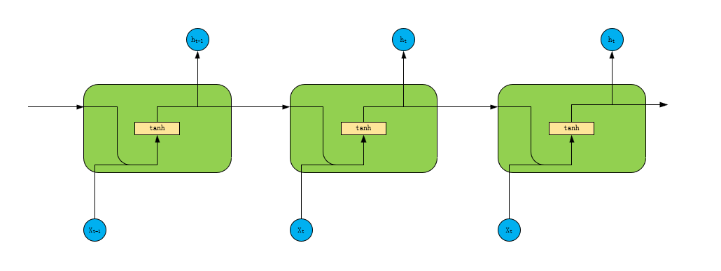
Figure 1: Structure of RNN.

As is shown in Figure 1, RNN is the simplest recurrent neural network. The output of the hidden layer at this instant is connected to both the input and the hidden layer output from the previous instant. The calculation process of RNN is very simple, with only one tanh layer.

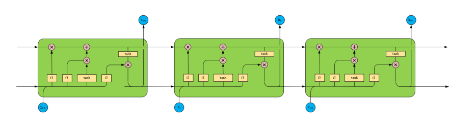
Figure 2: Structure of LSTM.

Figure 2 gives the structure of LSTM. LSTM is a type of RNN. Its current state is still connected to its former condition., but its structure is slightly more complex than traditional RNN. It has one more output state cell state than RNN, and the calculation is also slightly more complicated. LSTM solves the gradient vanishing/exploding problem of RNN.

3.2. LSTM Model Structure

A LSTM network is essentially made up of three main parts: an input gate, an output gate, and a forget gate. These elements are essential for the network to be able to remember and capture long-term dependencies in the data by selectively retaining or discarding information over extended sequences [11]. By selecting which new data to store, the input gate manages the information flow into the cell state. The forget gate aids the network in forgetting unnecessary information by deciding what data to remove from the cell state [12]. The ultimate output of the LSTM cell is produced by the output gate, which controls the information output from the cell state.

3.2.1. Forget Gate

In an LSTM network, the forgetting gate is essential for deciding which data to remove from the cell state. To achieve this, it applies a sigmoid activation function to each element in the cell state, producing a value between 0 and 1, which indicates how much of each piece of information should be remembered or lost.

The calculation formula for the forgetting gate is:

\( {f_{t}}=σ({W_{f}}∙[{h_{t-1}}, {x_{t}}] +{b_{f}}) \) (2)

By concatenating the current input \( {x_{t}} \) and the prior hidden state \( {h_{t-1}} \) , this formula determines the forget gate activation. A sigmoid activation function is then used. How much of each element in the cell state from the previous time step should be remembered or preserved is determined by the resulting forget gate vector.

3.2.2. Input Gate

This step is to add new memory information. The new memory information is obtained by multiplying the tanh unit by the weight. The calculation formula is as follows:

\( {i_{t}}=σ({W_{i}}∙[{h_{t-1}}, {x_{t}}] +{b_{i}}) \) (3)

\( {\widetilde{C}_{t}}=tanh({W_{c}}∙[{h_{t-1}}, {x_{t}}] +{b_{c}}) \) (4)

In a LSTM network, the forget gate output and the candidate values are combined to get the updated cell state by calculating how much of the new candidate values should be added to the cell state. The forget gate's output and the output of the tanh activation function, which represents the new candidate values, are multiplied element-wise in this combination. The following can be used as the calculation formula to update the cell state:

\( {C_{t}}={f_{t}}⊙{C_{t-1}}+{i_{t}}⊙{\widetilde{C}_{t}} \) (5)

To calculate how much of the previous state to keep, this formula multiplies the forget gate output element-by-element with the prior cell state. To calculate the amount of new data to add to the cell state, the input gate output is additionally multiplied element-wise by the new candidate values. The revised cell state is then calculated by adding these two terms.

3.2.3. Output Gate

The information to be output from the cell state to the following concealed state and to the network's output is determined by the output gate in an LSTM network. To regulate the information flow, it makes use of both the previous concealed state and the current input. There are two primary processes in the output gate calculation: creating the output gate vector and creating the output itself.

The calculation formula for the output gate at time step ( t ) can be expressed as:

\( {o_{t}}=σ({W_{o}}∙[{h_{t-1}}, {x_{t}}] +{b_{o}}) \) (6)

By concatenating the current input with the prior hidden state, this formula determines the output gate activation. A sigmoid activation function is then used. How much of the cell state should be output to the following concealed state and the network's output is determined by the output gate vector that results.

Once the output gate vector is obtained, the actual output \( {h_{t}} \) is computed by applying the output gate to the cell state:

\( {h_{t}}={o_{t}}⊙tanh({C_{t}}) \) (7)

In order to determine the output, this formula multiplies the element-wise values with the output gate vector after first applying the hyperbolic tangent activation function to the cell state. This procedure makes sure that only pertinent data from the cell state is transferred to the following hidden state and the output of the network.

3.3. Stock-Selecting Model Construction

Selecting stocks based on their expected yield involves analyzing historical data and applying predictive models to forecast future performance. To select the 10 stocks with the highest average expected yield in the next 10 trading days from April 11, 2016, to April 25, 2016, the following steps can be taken:

(1) Data Collection: Gather historical stock price data for a range of stocks for the specified time period (April 11, 2016, to April 25, 2016).

(2) Calculation of Expected Yield: A LSTM model is built using the T+1 period return rate as the regression object and the T-period factor value as the feature. The LSTM model is then utilized to forecast each stock's return rate for the upcoming period.

(3) Ranking: Calculate the average expected yield for each stock by averaging the expected yields for the next 10 trading days. Rank the stocks based on their average expected yield from highest to lowest.

(4) Selection: Select the top 10 stocks with the highest average expected yield for investment consideration.

(5) Validation: Validate the selected stocks and the predictive model used for estimation. This could involve backtesting the model on historical data to assess its accuracy and reliability.

By following these steps, we can identify and select the 10 stocks with the highest average expected yield for the specified time period, taking into account the limitations of computing power and the need for efficient analysis and decision-making.

4. Backtest Verification

The selected stocks are used as the portfolio to obtain the stock price return data from April 11, 2016 to April 25, 2016, and compared with 10 randomly selected stocks.

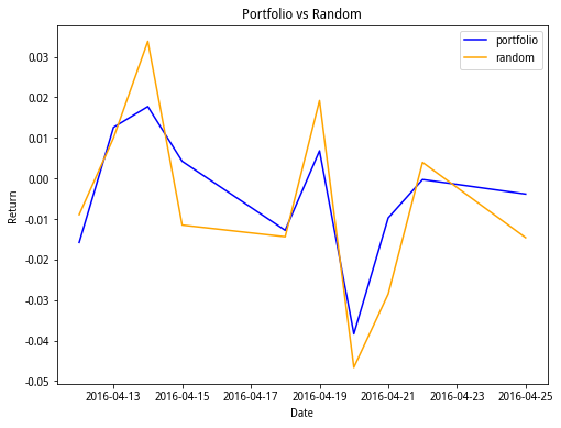
Figure 3: Backtest result.

Figure 3 gives the backtest result. It shows returns of two portfolios in ten trading days, one is the portfolio with stocks selected using the method proposed above which is named as ‘portfolio’ and the other is the portfolio with 10 randomly selected stocks which is named as ‘random’. Portfolio has better performance than random overall.

The average return of the selected stocks as portfolio is -0.40%, and the average return of the 10 randomly selected stocks as portfolio is -0.58%. This paper's proposed method is capable of effectively implementing stock selection. However, because of the limit of the compute power, the portfolio we choose have some room for improvement. The portfolio has negative return and its volatility is relatively high. That’s because there are only 45 candidate stocks. To improve our model, we can enlarge the candidate stock pool to get the portfolio having better performance.

5. Conclusion

The Information Criterion (IC) technique is used in the study as a filtering mechanism to sort through a large number of factors and determine which 11 are the most influential. The stock price is then used as the goal variable and these elements are used as input features to build a Long Short-Term Memory (LSTM) model for stock price forecasting. Recurrent neural networks (RNNs) of the LSTM type are good at identifying temporal dependencies in sequential data, which makes them appropriate for time series forecasting applications such as stock price prediction.

After building the LSTM model, the research moves on to establish a portfolio by choosing the top 10 stocks with the highest average returns. To ensure the portfolio's resilience and return-generating capability, this selection procedure probably takes historical performance, volatility, liquidity, and other pertinent variables into account.

A thorough backtesting process is carried out to confirm the suggested method's efficacy. Using historical data, the generated model and stock selection method are backtested to gauge their performance and potential for profit in real-world circumstances. This procedure offers empirical proof of the strategy's feasibility and promise for real-world implementation while reducing the risk of overfitting.

The results of the backtesting process validate the suggested method's effectiveness in stock picking. Through constant and superior performance when compared to alternative methods or benchmarks, the study validates the proposed approach's applicability and trustworthiness in the stock market trading setting.

Overall, the article uses cutting-edge methods from machine learning and quantitative finance to propose a methodical, data-driven approach for building portfolios and choosing stocks. It offers insightful information to investors looking to strengthen their decision-making procedures and boost portfolio performance in volatile financial markets through rigorous testing and empirical validation.

References

[1]. Song, Jialu. (2023). Research on Quantitative Stock Selection and Timing Strategy Based on Deep Learning. (Master's thesis). Nanjing University of Information Science & Technology.
[2]. Xiong, Geyi. (2024). Quantitative Stock Selection Model Based on Machine Learning Algorithms. (Master's thesis). Donghua University.
[3]. Li, Qianqian. (2019). Establishment and Optimization of Multi-factor Quantitative Stock Selection Model. (Master's thesis). Shandong University.
[4]. Bao, Xufan. (2023). Research on Quantitative Investment Strategy of Funds Based on Ensemble Learning. (Master's thesis). Soochow University.
[5]. Lei, Yuchen. (2023). Planning of Quantitative Stock Selection Scheme Based on Industry Factors. (Master's thesis). Shanghai Normal University.
[6]. Ding, Q. (2020). Research on Quantitative Investment Strategy of Stocks Based on Principal Component Analysis. Financial Times, (17), 74-76.
[7]. [Data Platform on 10JQKA]. (2024, 4 25). Retrieved from https://quant.10jqka.com.cn/view/dataplatform
[8]. Mo, Jiawei. (2024). Research on Stock Price Prediction and Stock Selection Strategy Based on LSTM Model. (Master's thesis). Guangzhou University.
[9]. Tang, Ruyi. (2022). Research on Optimization of Turtle Trading Model Based on LSTM Neural Network. (Master's thesis). East China Normal University.
[10]. Xu, Tianyu. (2024). Research on Quantitative Investment Portfolio Strategy Based on Sino-US Stock Markets. (Master's thesis). Zhejiang University of Science and Technology.
[11]. Ji, Churan. (2021). Research on Stock Index Price Prediction Based on LSTM Neural Network. (Master's thesis). Anhui University of Finance and Economics.
[12]. Ouyang, Fei. (2023). Research on Multi-factor Quantitative Investment Strategy Based on Machine Learning. (Master's thesis). Lanzhou University of Finance and Economics.
Cite this article
Yang,H. (2024). Application of Long Short-Term Memory (LSTM) in Multi-Factor Quantitative Investment Models. Advances in Economics, Management and Political Sciences,104,13-19.
Data availability
The datasets used and/or analyzed during the current study will be available from the authors upon reasonable request.
Disclaimer/Publisher's Note
The statements, opinions and data contained in all publications are solely those of the individual author(s) and contributor(s) and not of EWA Publishing and/or the editor(s). EWA Publishing and/or the editor(s) disclaim responsibility for any injury to people or property resulting from any ideas, methods, instructions or products referred to in the content.
About volume
Volume title: Proceedings of the 8th International Conference on Economic Management and Green Development
© 2024 by the author(s). Licensee EWA Publishing, Oxford, UK. This article is an open access article distributed under the terms and
conditions of the Creative Commons Attribution (CC BY) license. Authors who
publish this series agree to the following terms:
1. Authors retain copyright and grant the series right of first publication with the work simultaneously licensed under a Creative Commons
Attribution License that allows others to share the work with an acknowledgment of the work's authorship and initial publication in this
series.
2. Authors are able to enter into separate, additional contractual arrangements for the non-exclusive distribution of the series's published
version of the work (e.g., post it to an institutional repository or publish it in a book), with an acknowledgment of its initial
publication in this series.
3. Authors are permitted and encouraged to post their work online (e.g., in institutional repositories or on their website) prior to and
during the submission process, as it can lead to productive exchanges, as well as earlier and greater citation of published work (See
Open access policy for details).