1. Introduction

The financial industry is paying more attention to the quantification and mitigation of risk losses. Consequently, risk management theory is applied increasingly in financial markets.

Risk measure models for financial time series hold a significant position in modern financial research. Traditional risk measure methods, such as the variance-covariance approach and historical simulation, although effective to some extent, have shown limitations when dealing with nonlinear and non-normal distribution in financial time series. Therefore, numerous risk measure models have emerged in recent years, including Conditional Value at Risk (CVaR) and Extreme Value Theory (EVT). Alemany discusses the Classical kernel estimation (CKE) as also a better approach compared to empirical distribution which extrapolates above the maximum observed sample [1].

Value at Risk (VaR) and Expected Shortfall (ES) have become important measures of the market risk. Because VaR only needs to compute a quantile of a given distribution, all kinds of financial institutions use it as a practical tool to quantify risk. In estimating VaR, the main goal is to find a suitable distribution to describe the asset return [2]. VaR has also received a lot of criticism. Since it lacks subadditivity, the VaR of the portfolio may not always be less than the sum of the VaRs of the individual assets within the portfolio. Meanwhile, VaR only focus on quantile measure in certain confidence level and ignore the loss of tail after the quantile [3]. And ES concentrates on the expect value of loss after VaR and it is coherent. Therefore, this paper concerns VaR and ES to compare the different types of models.

The paper studies seven different models of three approaches in Time Series, the Parametric approach, Semi-parametric approach, and Non-parametric approach, and introduces a new concept Volatility of Deviation in VaR (VDVaR) to show the volatility in the difference of the actual number of violations and the expected number of violations. This paper uses VaR, ES, and VDVaR as indicators to analyze the accuracy and credibility of different models for risk measurement in different regions. Meanwhile, appropriate models are used to calculate the ES under different regions and take it as the stock index risk of the region. This research aims to conduct a comparative analysis of different models to evaluate their effectiveness in measuring risks across various regions and to provide more comprehensive tools for financial risk management.

2. Method

2.1. Data

Numerous risk models of parametric, semi-parametric, and non-parametric approaches have been demonstrated in the literature to predict VaR and ES. The effectiveness of these risk models is assessed by their capability to accurately represent the tail of the conditional loss distribution [4]. In the paper, these three approaches were applied to 4 market indices within 10 years in Emerging and Developed markets to assess each model in estimating VaR and ES at various confidence levels. Data is selected from the Shanghai SE Composite Index (SSE) in China, the Straits Times Index (STI) in Singapore, the SET Index in Thailand, and the S&P500 Index in America. All data are collected from investing.com. Investing.com offers real-time market data and analytical commentary on over 300,000 financial assets across more than 250 exchanges globally.

Let \( {X_{t}} \) be a daily negative log return on a financial asset price. The asset price is a close price on each day. Assume the dynamics of \( X \) is

\( {X_{t}}={μ_{t}}+{σ_{t}}{Z_{t}}, \) (1)

where innovation \( {Z_{t}} \) is a white noise process that follows an independent and identically distributed (i.i.d.) pattern with a mean of zero and unit variance. This research only focuses on a single asset, so the cumulative distribution function (cdf) of \( Z \) is one dimension \( {F_{Z}}(z) \) . This paper is concerned with the 1-step predictive distribution in VaR and ES. Therefore, the measures are easy to get

\( VaR_{q}^{t+1}={μ_{t+1}}+{σ_{t+1}}{z_{q}}, \) (2)

\( ES_{q}^{t+1}={μ_{t+1}}+{σ_{t+1}}E[Z|Z \gt {z_{q}}], \) (3)

where \( {z_{q}} \) is the upper q-th quantile of \( {F_{Z}}(z) \) . Because of one step forecast, this research uses \( ({X_{t-n+1}},{X_{t-n+2}},…,{X_{t}}) \) n days data to predict \( {X_{t+1}} \) and so on. For consistency, the value of n is fixed, and make it equal to 1000.

Augmented Dickey Fuller (ADF) Test is used to test for detecting stationarity in time series samples. The ADF test is an improved version of the Dickey-Fuller test that extends by adding a higher-order regression process to the model. Dickey-Fuller test tests for unit-root nonstationarity. It tests the suitability of the data for fitting with a time series model. If a unit root is present, it indicates that the series behaves more like a stochastic process rather than a typical time series. This is the first step in testing before fitting the model [5]. In all four sets of data studied in this paper, the p-value of the ADF test is less than 0.01, which means that there is no unit root and the data is stationarity.

2.2. Approach and Model

2.2.1. Parametric Approach

In the first method, the paper uses the Auto-Regressive Moving Average (ARMA)-GARCH Model with the ARMA(1,1)-GARCH(1,1) process

\( {X_{t+1}}={μ_{r}}+ϕ({X_{t}}-{μ_{r}})+θ{ϵ_{t}}+{ϵ_{t+1}}, \) (4)

\( σ_{t+1}^{2}=ω+αϵ_{t}^{2}+βσ_{t}^{2}, \) (5)

which is direct and effective way and easy to modify with other approaches. ARMA model is aimed to get conditional mean and GARCH model is used to get volatility. To implement the model, a certain innovation distribution like the Gaussian distribution must be chosen. Cont emphasizes the inadequacy of Gaussian models in capturing the leptokurtic and heavy-tailed nature of financial data [6]. Therefore, this paper uses two distributions, one is Gaussian distribution and the other is Student’s t-distribution which is more leptokurtic than Gaussian distribution.

The model can be fitted with maximum likelihood (ML) method. The estimate of parameters can be obtained \( (\hat{ϕ},\hat{θ},\hat{ω},\hat{α},\hat{β}) \) . Conditional mean \( ({μ_{t-n+1}},{μ_{t-n+2}},…,{μ_{t}}) \) and volatility \( ({σ_{t-n+1}},{σ_{t-n+2}},…,{σ_{t}}) \) series can be determined by these parameters. To check if the model fit well, residual series

\( ({z_{t-n+1}},…,{z_{n}})=(\frac{{x_{t-n+1}}-\hat{{μ_{t-n+1}}}}{\hat{{σ_{t-n+1}}}},…,\frac{{x_{t}}-\hat{{μ_{t}}}}{\hat{{σ_{t}}}}) \) (6)

should be independent each other. For day t+1, the one step forecast is used to estimate conditional mean

\( {μ_{t+1}}={μ_{r}}+\hat{ϕ}({X_{t}}-{μ_{r}})+\hat{θ}\hat{{ϵ_{t}}} \) (7)

and variance

\( {σ_{t+1}}=\hat{ω}+\hat{α}\hat{ϵ_{t}^{2}}+\hat{β}\hat{σ_{t}^{2}}, \) (8)

where \( \hat{{ϵ_{t}}}={X_{t}}-\hat{{μ_{t}}} \) . In Gaussian innovation distribution, \( {z_{q}} \) can be estimated \( Φ(q) \) . And in t innovation distribution

\( {z_{q}}=\sqrt[]{(v-2)/v}F_{T}^{-1}(q). \) (9)

Finally, in this paper, it is checked that in the ARMA-GARCH model, the residuals \( {Z_{t}} \) comply with the previously mentioned assumption that it is a white noise process. The Ljung-Box test is used, and the first 1000 days ARMA-GARCH model shows that the p values of S&P500, STI, SSE, and SET are 0.633, 0.944, 0.666, and 0.502. The residuals seem to be iid and several Ljung-Box tests were also carried out over selected time periods, and it was determined that there was no evidence contradicting the i.i.d. assumption for the residuals.

2.2.2. Semi-Parametric Approach

The second method combines the Parametric approach and the Semi-parametric approach. Re-fitting the tail distribution based on the first approach. Mcneil and Frey modify the ARMA-GARCH model with extreme value theory (EVT) [7]. They keep the main body of the innovation distribution unchanged and change the tail distribution to the generalized Pareto distribution (GPD) to better capture extreme loss situations in financial markets. The formula of GPD is as follows

\( {G_{ξ,β}}\begin{cases} \begin{array}{c} 1-{(1+\frac{ξx}{β})^{-\frac{1}{ξ}}} if ξ≠0 \\ 1-{e^{-\frac{x}{β}}} if ξ=0 \end{array} \end{cases}, \) (10)

where \( β \gt 0 \) and if \( ξ \lt 0, 0≤x≤-β/ξ \) , if \( ξ≥0, x≥0 \) . And x is excess residuals over the threshold which means \( x=z-μ \) , where z is residual above the threshold and \( μ \) is the threshold. Threshold selection is critical. Smith has indicated that the procedure to calculate maximum likelihood estimates (MLE) \( \hat{ξ},\hat{ β} \) is asymptotically unbiased if \( μ→{x_{0}} \) , where \( {x_{0}} \) is the right endpoint of residual series [8]. So it cannot be too small. The Hill estimator is another way to calculate estimators, but this method is not stable and if the threshold is too small, the mean squared error (MSE) and bias can be very large [7]. This paper uses robust method MLE and if the choice of threshold is too large, the MLEs are worse than Hill estimators.

Let resort the residual series with decreasing order \( {z_{(1)}}≥{z_{(2)}}≥…≥{z_{(n)}} \) , the threshold is \( {z_{(k+1)}} \) , the (k+1)th order residual. This means there are n residual over threshold. The \( k \) should be much larger than n. In this paper, \( k \) is 80. For \( q \gt 1-k/n \) [7],

\( \hat{{z_{q}}}={z_{(k+1)}}+\frac{\hat{β}}{\hat{ξ}}({(\frac{1-q}{k/n})^{-\hat{ξ}}}-1), \) (11)

\( E[Z|Z \gt {z_{q}}]=\hat{{z_{q}}}(\frac{1}{1-\hat{ξ}}+\frac{\hat{β}-\hat{ξ}{z_{(k+1)}}}{(1-\hat{ξ})\hat{{z_{q}}}}). \) (12)

There are total N data and use the amount of n to fit the model, where \( N \gt n \) . The predictive interval PI is \( [n+1,n+2,...,N] \) . On each day \( t∈PI \) , a new ARMA(1,1)-GARCH(1,1) model is fitted and GPD tail estimators are recalculated.

2.2.3. Non-Parametric Approach

In this method, the paper does not make any assumptions. The first model is the Empirical distribution model. VaR is 95% quantile of \( ({X_{t-n+1}},{X_{t-n+2}},…,{X_{t}}) \) and ES is the sample average of series which X is larger than VaR. The estimate cdf of empirical distribution is

\( \hat{F}(x)=\sum _{i=1}^{n}I({X_{i}}≤x). \) (13)

Alemany shows that empirical distribution cannot extrapolate beyond the highest data point observed and it only collects data less than x to construct \( F(x) \) [1]. If the sample data is not large over some time. Then the VaR and ES predicted based on the empirical distribution may deviate greatly from the actual situation, resulting in huge potential losses in the future. Therefore, a new model kernel density estimation (KDE) is added

\( \hat{F}(x)=\sum _{i=1}^{n}K(\frac{x-{X_{i}}}{b}), \) (14)

where \( K(·) \) is the cdf of kernel function and b is bandwidth. In this paper \( K(·) \) is the cdf of gaussian kernel function. For bandwidth, this research uses cross-validation approach to minimize an error criterion. KDE is more flexible because it uses all data larger or smaller than \( x \) .

For backtesting the ES, the estimate volatility \( \hat{{σ_{t+1}}} \) need to be calculated. In this approach, the paper uses the standard deviation of the latest thirty days of data in a given period as the \( \hat{{σ_{t+1}}} \) .

2.3. Volatility of Deviation in VaR

This paper introduces a new concept to evaluate the accuracy of various risk prediction models. The rest of the days \( t∈PI \) are divided into 5 stages. For 95% VaR, expected violations \( (e{v_{1}},…,e{v_{5}}) \) is 0.05 times the amount of data in each stage. Actual violations \( (a{v_{1}},…,a{v_{5}}) \) in each stage are the number of events occur when \( {x_{t+1}} \gt VaR_{0.95}^{t+1} \) . And the deviation in this each stage is \( (a{v_{1}}-e{v_{1}},…,a{v_{5}}-e{v_{5}}) \) . Volatility of Deviation is the standard deviation of this series. VDVaR can be used to measure whether the amount of violation is evenly distributed across time. If the value of VDVaR is too large, violation incidents may erupt at a certain stage, and the number of violations in different stages may vary significantly. It leads to inaccurate predictions in the short term.

3. Result

This paper uses t innovation distribution in a semi-parametric approach because normal distribution has a large probability of underestimating the tail loss and leads to a bad ES. The GRACH type can be changed with IGARCH and GJR-GARCH. Glosten shows that the GJR-GARCH model considers that conditional volatility is affected by positive and negative shocks [9]. Due to the asymmetry, this model is usually able to predict asset price volatility more accurately than the standard GARCH model. The IGARCH model assumes persistence \( \hat{α}+\hat{β}=1 \) . Therefore, none of the other results, such as unconditional variance or half-life, can be computed, and the impact of past data on future volatility decays very slowly [10]. This proves that the IGARCH model has good stability.

The paper backtests the models on four historical series of negative log returns. In VaR, the amount of violation in each model and binomial test p-value are shown. Bootstrap Hypothesis Test p value is indicated in ES and VDVaR is listed at the end.

3.1. VaR

Tables 1 and 2 show the backtesting results with 95% and 99% VaR. In Table 1, the Gaussian innovation distribution outperforms t innovation distribution, but in Table 2 vice versa. The results of the combination of semi-parametric and parametric approaches are better than only the parametric approach in most cases. Exceptions are made in the SSE index in Table 1, STI and SSE index in Table 2. The EVT_GJRGARCH model has robust results both at 95% and 99% Quantile. The EVT_GARCH and EVT_IGARCH models have some excellent results in some cases. As in Table 1, both of their p value in the SET index are 1 and EVT_GARCH also have a perfect p-value in the SET index in Table 2. But there are times when both models give very outrageous results. For example, in a 99% Quantile situation, EVT_GARCH only has a 0.041 p-value in the STI index which is worse than the Gaussian distribution and it's unacceptable. In the Non-parametric approach, Empirical distribution has a good result when q=0.95, and the Kernel density estimator seems that it cannot fit the actual situation well. But if q=0.99, the KDE shows p-value is high enough to trust except the S&P500 and the accuracy of empirical distribution is not as good as before.

Table 1: Backtesting Results with 95% VaR: number of violations obtained using three approaches. Binomial test p-values are given in brackets.

Table 2: Backtesting Results with 99% VaR: number of violations obtained using three approaches. Binomial test p-values are given in brackets.

3.2. ES

Tables 3 and 4 show the backtesting results with 95% and 99% ES. In both tables, the p-value of the Gaussian innovation distribution is too small and the fit is very poor. This also confirms the previous conclusion that a Gaussian distribution underestimates the tail distribution of the loss. In contrast, the t-distribution demonstrates very good results in all cases. EVT_GJRGARCH maintains its very robust nature and all results are acceptable in 95% and 99% Quantile. In Table 3, EVT_GARCH performs not good with SSE index and in Table 4, EVT_IGARCH cannot fit STI index very well. In the non-parametric approach, when q=0.95, Empirical distribution has a good result in VaR but shows a bad p value in ES. When q=0.99, the result of ES is enough to accept, but those of VaR are not as precise. The results of KDE are the opposite of Empirical distribution.

Table 3: Backtesting Results with 95% ES: p-values for bootstrap test

Table 4: Backtesting Results with 99% ES: p-values for the bootstrap test

3.3. VDVaR

Tables 5 and 6 show VDVaR in different quantities. The results of the combination of semi-parametric and parametric approaches are not much different in most cases. However, the volatilities of the non-parametric approach are much more than other approaches. This also demonstrates that the non-parametric approach can have a period where the number of violations is much higher or lower than expected. High volatility reduces the accuracy of model predictions. Meanwhile, the overall trend in volatility is downward as the quantile increases.

Table 5: Volatility of Deviation in 95% VaR

Table 6: Volatility of Deviation in 99% VaR

4. Discussion

This paper uses backtesting VaR, ES, and backtesting VDVaR as the three criteria for selecting models. When choosing a suitable model, one should not just look at a single metric, but analyze it comprehensively. Gaussian innovation distribution performs well in 95% VaR. Since it has a light tail, this model does not capture the extremes of the tail well, which results in a poor p-value for the ES. T innovation distribution has a good fit in 95% ES. However, the 95% VaR predicted by this model has so far deviation from the actual situation that it has been rejected. The EVT_GJRGARCH model can estimate very robust results in most cases. This also indicates its strong applicability. The EVT model can obtain reliable results by changing the GARCH type. The combination of semi-parametric and parametric approaches has great flexibility and can switch the appropriate model according to different data to obtain a good fit. The non-parametric approach can also be calculated with enough trust in some cases. However, the values of VDVaR are very high, so it should be prudent when choosing this type of model. If the VDVaR value is too large, it leads to overestimation or underestimation of the risk value over some time.

95% ES is used as a measure of equity index risk for the four regions and select the four most appropriate models based on the previous data. The paper chooses the EVT IGARCH model for S&P500 and STI, the EVT GJRGARCH model for SSE, and the standard EVT GARCH model for SET. Figure 1 as follows shows their risk measurement. The x-axis means time and the y-axis means ES. For peaks, the U.S. S&P500 is well ahead of the rest of the index. Then comes Thailand's SET and Singapore's STI. China’s SSE does not show a significant peak. For non-peak, S&P500 and SSE consistently have relatively high ES. And for most of the time, the ES of STI and SET are relatively low.

Figure 1: Risk Measure with 95% ES (Original).

Figure 2 shows the 99% ES as a measure of equity index risk. The left picture (a) shows the ES of the empirical distribution model and KDE model with STI index. The KDE model shows more flexible and include more extreme loss than empirical distribution model. Therefore, KDE model is chosen for STI and apply EVT GJRGARCH model for S&P500, t innovation distribution ARMA-GARCH model for SSE and EVT IGARCH model for SET. In the right picture (b), the ES value of the S&P500 is relatively high at both peak and non-peak levels. Except for peak values, the ES of SET is very low in other stages. China’s SSE does not show a significant peak as before, but its ES value decreases in the latter stage. ES of STI is much more different than others. KDE model is more flexible and contain more extreme loss, but it looks like flatter than time series model. ES of STI never shows a significant peak period. This also represents in peak stage, the KDE model's predictions are much lower than the actual situation, and a large number of violations occur. However, due to the impact of extreme losses, the ES after the peak stage is also relatively high, which can better avoid the occurrence of violations. Overall, the non-parametric approach is a simple and effective method during non-peak periods, but once a large shock event occurs, the concentrated outbreak of extreme losses can also render the model ineffective.

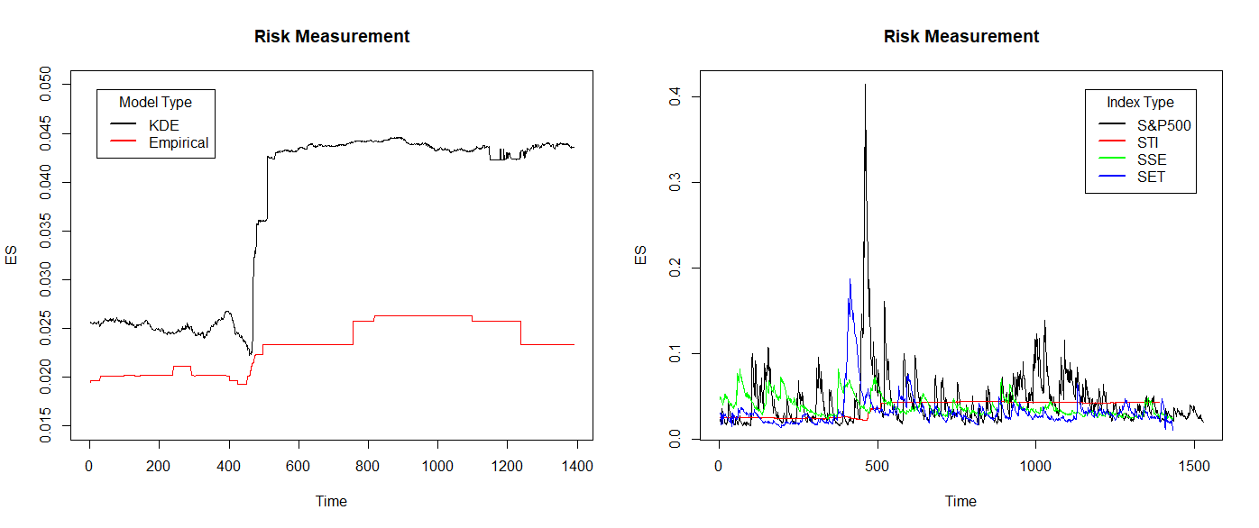
Figure 2: Risk Measure with 99% ES. (a) ES of empirical distribution model and KDE model with STI index; (b) Risk Measure in four appropriate models with 99% ES (Original).

5. Conclusion

This paper researches the performance of three approaches to analyze the risk measures in different regions and focuses on two extreme qualities 0.95 and 0.99. The author proposed a new concept VDVaR, and used it along with, backtesting VaR and backtesting ES as three criteria to check the fit of the seven models.

The paper shows that the Gaussian innovation distribution model does not fit the risk well. Even if some 95% VaR predictions are good, the corresponding ES predictions are not trustworthy enough. And t innovation distribution model can be used optionally. In a 99% quantile situation, this model can be a good fit for some specific indexes like STI and SSE. The method which combines parametric and semi-parametric approaches is flexible. GARCH-type can be changed so that it can be used in most cases. VDVaR is mainly used to test the non-parametric approach. Because in some cases, the empirical distribution model or KDE model can estimate VaR and ES well. However, after adding VDVaR, the number of violations that deviate from the expected value is quite volatile. This means that even if the overall prediction results are credible, the prediction results at some local stages may deviate seriously from the actual situation. Therefore, it is important to compare the criteria thoroughly when choosing this type of model. Finally, the paper visualizes the equity index risk across countries and compares the risk condition across countries in peak and off-peak scenarios.

This paper researches risk measure approaches of one-dimensional financial assets in a step forecast. As for future research directions, multiple-day forecasts and multiple-dimension portfolios should be studied. This allows for further exploration of the credibility and effectiveness of different models and methods in more complex situations.

References

[1]. Alemany, R., Bolancé, C., & Guillen, M. (2013). A nonparametric approach to calculating value-at-risk. Insurance: Mathematics and Economics, 52(2), 255-262.
[2]. Chang, Y. P., Hung, M. C., & Wu, Y. F. (2003). Nonparametric estimation for risk in value-at-risk estimator. Communications in Statistics-Simulation and Computation, 32(4), 1041-1064.
[3]. Righi, M., & Ceretta, P. S. (2013). Individual and flexible expected shortfall backtesting. Journal of Risk Model Validation, 7(3), 3-20.
[4]. James, R., Leung, H., Leung, J. W. Y., & Prokhorov, A. (2023). Forecasting tail risk measures for financial time series: An extreme value approach with covariates. Journal of Empirical Finance, 71, 29-50.
[5]. Dickey, D. A., & Fuller, W. A. (1979). Distribution of the estimators for autoregressive time series with a unit root. Journal of the American statistical association, 74(366a), 427-431.
[6]. Cont, R. (2001). Empirical properties of asset returns: stylized facts and statistical issues. Quantitative finance, 1(2), 223.
[7]. McNeil, A. J., & Frey, R. (2000). Estimation of tail-related risk measures for heteroscedastic financial time series: an extreme value approach. Journal of empirical finance, 7(3-4), 271-300.
[8]. Smith, R. L. (1987). Estimating tails of probability distributions. The annals of Statistics, 1174-1207.
[9]. Glosten, L. R., Jagannathan, R., & Runkle, D. E. (1993). On the relation between the expected value and the volatility of the nominal excess return on stocks. The journal of finance, 48(5), 1779-1801.
[10]. Engle, R. F., & Bollerslev, T. (1986). Modelling the persistence of conditional variances. Econometric reviews, 5(1), 1-50.
Cite this article
Yuan,S. (2024). Comparative Analysis of Risk Measure Model in Financial Time Series. Advances in Economics, Management and Political Sciences,107,94-103.
Data availability
The datasets used and/or analyzed during the current study will be available from the authors upon reasonable request.
Disclaimer/Publisher's Note
The statements, opinions and data contained in all publications are solely those of the individual author(s) and contributor(s) and not of EWA Publishing and/or the editor(s). EWA Publishing and/or the editor(s) disclaim responsibility for any injury to people or property resulting from any ideas, methods, instructions or products referred to in the content.
About volume
Volume title: Proceedings of ICFTBA 2024 Workshop: Finance's Role in the Just Transition
© 2024 by the author(s). Licensee EWA Publishing, Oxford, UK. This article is an open access article distributed under the terms and
conditions of the Creative Commons Attribution (CC BY) license. Authors who
publish this series agree to the following terms:
1. Authors retain copyright and grant the series right of first publication with the work simultaneously licensed under a Creative Commons
Attribution License that allows others to share the work with an acknowledgment of the work's authorship and initial publication in this
series.
2. Authors are able to enter into separate, additional contractual arrangements for the non-exclusive distribution of the series's published
version of the work (e.g., post it to an institutional repository or publish it in a book), with an acknowledgment of its initial
publication in this series.
3. Authors are permitted and encouraged to post their work online (e.g., in institutional repositories or on their website) prior to and
during the submission process, as it can lead to productive exchanges, as well as earlier and greater citation of published work (See
Open access policy for details).