


1. Introduction
On April 15, 1912, the British luxury passenger ship Titanic sank on its maiden voyage from Southampton to New York because of a collision with an iceberg, resulting in the death of 1502 out of 2224 passengers and crew, which is one of the most famous tragedies in modern history [1]. Various approaches have been explored to analyze the titanic data. For instance, Logistic Regression, K Nearest Neighbors, Naive Bayes, Support Vector Machines, Decision Tree, Bagging, Extra Trees, Random Forest, Gradient Boosting. F-measure scores are used to show how the model performed [1]. Another similar research, using artificial neural networks and distinct data presentations, attaining high accuracy more than 99% [2].
Thus, this paper will use the approaches of logistic regression, decision tree, random forest and hard voting to build a model based on the given dataset to predict whether the targets survived or not in this tragedy. Moreover, this article aims to gain insights into the factors that influence the survival rate of passengers and establish a model to predict what sort of people are more likely to survive this catastrophe is the objective of the article, helping more people who encounter danger on board in the future.
The remaining of this paper is as follows. Section 2 is creating useful variables to make the dataset more complete by feature engineering and identifying the variables that influence the survival rate through data visualization. Section 3 is developing hard voting system including logistic regression, decision tree and random forest. Section 4 is Evaluating the models through accuracy, confusion matrix, ROC curve, etc.
2. Data
2.1. Data source and variables
Two data sets from Kaggle are given: a training set and a test set. The training set and test set are used together to perform data cleaning as more information can be inferred from the data. There are 12 variables in the training set (PassengerId, Survived, Pclass, Name, Sex, Age, SibSp, Parch, Ticket, Fare, Cabin, Embarked). The test set does not contain Survived. From the missing map, several missing values lies in the dataset. There are 263 missing in Age, 2 in Embarked, 1014 in Cabin and 1 in Fare. Various methods are utilized to tackle this.
2.2. Feature engineering
2.2.1. Title
Name consists of the first name, the last name and the title, it's worth to find how different titles influence the survival rate. So, title is separated and created a new variable called Title, there are some repeating titles and rare titles that are condensed into Title_short for better categorize, which only contains master, Miss., Mrs., Mr., and others [3].
2.2.2. Ticket
It is obvious that there are some passengers with the same ticket number, so the numbers are calculated and put into a variable called ticket_u. ticket_u is the unique number of ticket numbers [4].
2.2.3. Fare level
The distribution of the ticket fare illustrates that the majority of passengers pay 8 on the fare and small groups of passengers pay more or less, there may be a relationship between fare level, Pclass and Survived so that Fare is categorized into 3 groups: expensive, middle, cheap. As shown in figure 1, passengers with expensive fares are more likely to be in higher class which represents social states.
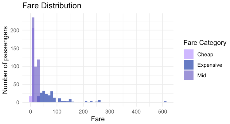
Figure 1: Ticket fare distribution
2.2.4. Child & Adult
Age is separated into child (less than 18 years old) and adult (greater or equal to 18) because survival rate may be related to whether they are adults or not.
2.2.5. Mother & Not mother
It is possible to classify the passengers by whether this person is a mother or not. Some mothers may prioritize protecting their children. So, the passenger who is female and greater than 18 and has a parch greater than 0 and whose title is not miss would be a mother.
2.3. Data visualization
2.3.1. Age, Sex & Survival
As shown in figure 2, male dies significantly more than females. This can be attributed to social norms that the male who died was perceived as a hero. Women approximately aged between 10 and 50 have greater chances to survive resulted from that they have more energy to escape than children and the elderly.
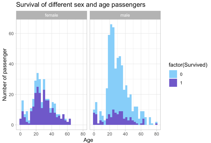
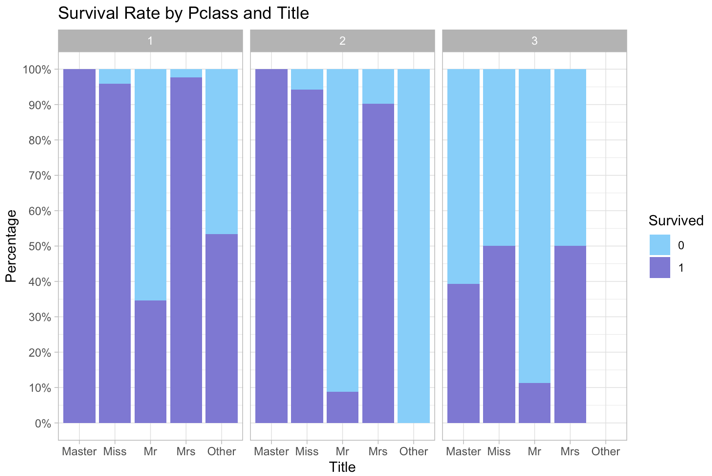
Figure 2: Survival of different sex and age passengers Figure 3: Survival rate by Pclass and Title
2.3.2. Pclass, Title & Survival
From figure 3, with higher Pclass, passengers are more likely to survive because they are closer to the deck in which lifeboats are placed. Also, they can have more information about the boat because they have high social status and may know the crews on the boat [4]. Title Mr. die more and Master, Miss., Mrs. die less because Masters have high skills and may be useful for society.
2.3.3. Fare level, Sex & Survival
Figure 4 illustrates that passengers who pay more for their tickets will survive more as they are wealthy and have high social classes so that they will be in higher passenger classes and as above, can survive. In mid fare level, the number of passengers is the highest and the death probability is higher than the survival probability. Nevertheless, the survival proportion in cheap fare levels is much lower than others.
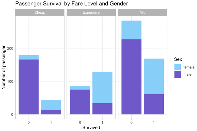
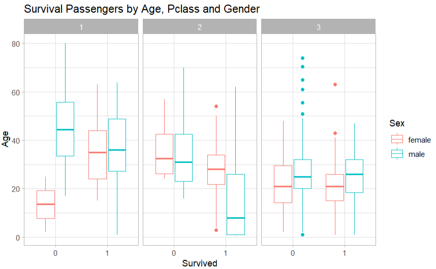
Figure 4: Passenger survival by fare level and gender | Figure 5: Survival passengers by Age, Pclass and Gender |
2.3.4. Pclass, Age, Sex & Survival
The fact that almost all the females from Pclass1 and Pclass2 survived and the proportion of males in the Pclass3 who lost their lives and who survived are almost the same in figure 5. On average, Pclass1 passengers aged around 35 are more likely to survive while lower-age passengers survived in classes 2 and 3.
3. Methodology
The basic idea is that a hard vote system is developed which consists of two logistic models, 2 decision tree models and a random forest, which is shown on figure 6. It gets prediction separately from these 5 models and chooses their major prediction which is survived or died. The sub-models have different algorithms and explanatory variables. For logistics, stepwise and forward stepwise are adopted while there is a change in maximum depth and algorithm in decision trees.
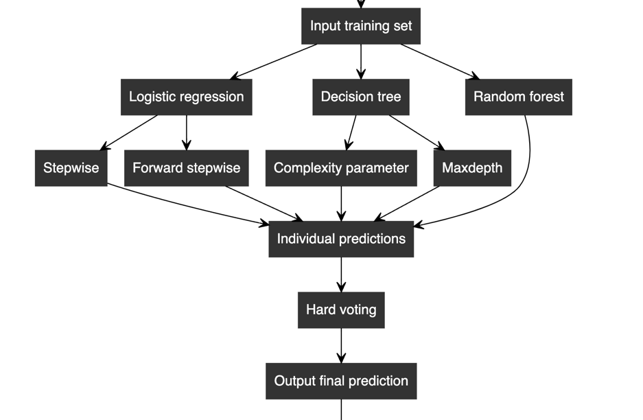
Figure 6: Model overview
3.1. Assumptions
Assumption 1: The explanatory variables are independent [5].
Correlation coefficients between numerical variables are calculated. In the correlation matrix, some of the variables have high r, implying that multicollinearity occurs. This can be attributed to variables that are deduced from each other or there is some similarity between them. For instance, Parch and FamilySize have r of 0.79 and this may be because family size also includes people from Parch [6].
Assumption 2: There is no multicollinearity among explanatory variables [5].
Chi-square tests for checking the independence of categorical variables are carried out. The null hypothesis is that two variables are independent and alternative hypothesis is that two variables are not independent. The p-values of the test are all smaller than 0.05. Thus, reject the null hypothesis and accept the alternative one which is the categorical variables may be associated [6]. These results may indicate some decrease in precision in the model [7].
Assumption 3: Explanatory variables and log odds of response variable has linear relationship [5].
3.2. Logistic regression
Regression is employed as a method of finding the relationship between explanatory variables and Survival, making predictions based on that relationship [8]. As Survival is a binary categorical data consisting of 0 and 1, logistic regression is adopted to map the original data into 0 to 1 interval using a logistic function and translates it into dummy variables.
3.3. Decision tree
Decision tree is a tree-like, hierarchical flowchart that lists the possible outcomes and makes decisions. Decision tree is used to predict the Survival based on choosing different variables as separating criteria. Classification tree is chosen as the response variable is categorical [9].
3.4. Random forest
Random forest is an ensemble learning model which consists of several decision trees. The model employs random feature selection to ensure that different trees focus on different features. It creates bootstraps and uses bagging to make decisions [10].
3.5. Hard voting
The models above are combined into a bigger one to make precise decisions. By collecting predictions of these models, it is able to calculate number of 1s and 0s of a particular passenger. If number of 1s are larger than number of 0s for a particular passenger, then the final prediction will be 1. So, the model takes the majority votes of each individual model and gives out a more objective prediction [11].
4. Results and analysis
4.1. Logistic regression
The model with all variables (Pclass, Sex, Age, SibSp, Parch, Fare, Embarked, Title_short, FamilySize, Fare_level, ticket_u, Child_adult, Mother) and with a stepwise algorithm is adopted first. After applying the algorithm, it remains the variables: Pclass, Sex, Age, SibSp and Title_short. They all have a negative correlation with survival.
Table 1: Summary of original logistic regression
Estimate | Std.error | z value | Pr(>|z|) | |
Intercept | 19.728467 | 503.690869 | 0.039 | 0.968757 |
Pclass | -1.246371 | 0.147528 | -8.448 | < 2e-16 |
Sexmale | -14.592789 | 503.690400 | -0.029 | 0.976887 |
Age | -0.017617 | 0.008901 | -1.979 | 0.047804 |
SibSp | -0.585807 | 0.128495 | -4.559 | 5.14e-06 |
Title_shortMiss | -15.043507 | 503.690687 | -0.030 | 0.976173 |
Title_shortMr | -3.426276 | 0.570379 | -6.007 | 1.89e-09 |
Title_shortMrs | -14.692372 | 503.690740 | -0.029 | 0.976729 |
Title_shortOther | -2.916660 | 0.823481 | -3.542 | 0.000397 |
Table 2: VIF of original logistic regression
GVIF | DF | GVIF^(1/(2*Df)) | |
Pclass | 1.494027e+00 | 1 | 1.222304 |
Sex | 5.910247e+06 | 1 | 2431.099922 |
Age | 1.779851e+00 | 1 | 1.334110 |
SibSp | 1.545337e+00 | 1 | 1.243116 |
Title_short | 1.087538e+07 | 4 | 7.578016 |
P-value for Sexmale and Title_shortMiss and Title_shortMrs are greater than 0.05 and the standard error is 504 which is very large. This reflects that the data spread out and there is multilinearity between variables. Variance inflation factor for Sex is the highest and the Title_short is also higher than 5, which indicates the multicollinearity.
Since there is multicollinearity between Sex and Title, and the VIF of Sex is the greatest, Sex is deleted first from the model. After applying the logistic regression, there is no large standard error in the model and the accuracy is 85.39%.
Table 3: Summary of logistic regression with Sex deleted
Estimate | Std. Error | z value | Pr(>|z|) | |
Intercept | 5.174151 | 0.722207 | 7.164 | 7.81e-13 |
Pclass | -1.258066 | 0.147616 | -8.523 | < 2e-16 |
Age | -0.018078 | 0.008882 | -2.035 | 0.04182 |
SibSp | -0.586628 | 0.128200 | -4.576 | 4.74e-06 |
Title_shortMiss | -0.447870 | 0.529721 | -0.845 | 0.39784 |
Title_shortMr | -3.426427 | 0.570780 | -6.003 | 1.94e-09 |
Title_shortMrs | -0.094700 | 0.576396 | -0.164 | 0.86950 |
Title_shortOther | -2.525146 | 0.773287 | -3.265 | 0.00109 |
Table 4: VIF of logistic regression with Sex deleted
GVIF | DF | GVIF^(1/(2*Df)) | |
Pcalss | 1.516358 | 1 | 1.231405 |
Age | 1.791430 | 1 | 1.338443 |
SibSp | 1.541600 | 1 | 1.241612 |
Title_short | 2.126826 | 4 | 1.098921 |
Table 5: Confusion matrix of logistic regression with Sex deleted
Actual: 0 | Actual: 1 | |
Predicted: 0 | 100 | 10 |
Predicted: 1 | 16 | 52 |
Furthermore, a forward stepwise selection is used instead of stepwise. Step forward starts with one variable inside and adds 1 variable in 1 step until there is no more variable with a significant p-value. Sex is deleted and according to the results, FamilySize is also deleted. So, this model gives more final variables than the previous one and higher accuracy of 86.52%.
Table 6: Summary of forward stepwise logistic regression
Estimate | Std. Error | z value | Pr(>|z|) | |
Intercept | 4.6610184 | 1.1806777 | 3.948 | 7.89e-05 |
Pclass | -1.0543620 | 0.2038324 | -5.173 | 2.31e-07 |
Age | -0.0197938 | 0.0101824 | -1.944 | 0.051904 |
SibSp | -0.6240889 | 0.1664320 | -3.750 | 0.000177 |
Parch | -0.2267935 | 0.2059312 | -1.101 | 0.270763 |
Fare | -0.0006696 | 0.0032382 | -0.207 | 0.836175 |
EmbarkedQ | 0.0868287 | 0.4391450 | 0.198 | 0.843262 |
EmbarkedS | -0.4161086 | 0.2769700 | -1.502 | 0.133004 |
Title_shortMiss | -0.5119173 | 0.5499646 | -0.931 | 0.351947 |
Title_shortMr | -3.4640068 | 0.6038896 | -5.736 | 9.68e-09 |
Title_shortMrs | -0.0061794 | 0.6644041 | -0.009 | 0.992579 |
Title_shortOther | -2.6989577 | 0.8028655 | -3.362 | 0.000775 |
Fare_levelExpensive | 0.9168914 | 0.5263071 | 1.742 | 0.081487 |
Fare_levelMid | 0.4127757 | 0.3352569 | 1.231 | 0.218240 |
ticket_u | 0.0119990 | 0.1281993 | 0.094 | 0.925430 |
Child_adultChild | -0.0698105 | 0.4145554 | -0.168 | 0.866270 |
MotherNot Mother | 0.0948320 | 0.6475193 | 0.146 | 0.883563 |
Table 7: VIF of forward stepwise logistic regression
GVIF | DF | GVIF^(1/(2*Df)) | |
Pclass | 2.803733 | 1 | 1.674435 |
Age | 2.296802 | 1 | 1.515520 |
SibSp | 2.522266 | 1 | 1.588164 |
Parch | 2.588749 | 1 | 1.608959 |
Fare | 2.144779 | 1 | 1.464506 |
Embarked | 1.509280 | 2 | 1.108390 |
Title_short | 5.002462 | 4 | 1.222920 |
Fare_level | 3.538732 | 2 | 1.371551 |
ticket_u | 4.281335 | 1 | 2.069139 |
Child_adult | 2.379662 | 1 | 1.542615 |
Mother | 2.647663 | 1 | 1.627164 |
Table 8: Durbin-Watson Test of forward stepwise logistic regression
lag | Autocorrelation | D-W Statistics | p-value |
1 | 0.02084805 | 1.957897 | 0.624 |
Table 9: Confusion matrix of forward stepwise logistic regression
Actual: 0 | Actual: 1 | |
Predicted: 0 | 101 | 9 |
Predicted: 1 | 15 | 53 |
Receiver Operating Characteristics (ROC) curve is used to visualize the result, the true positive rate is the sensitivity of the model and the false positive rate is the specificity of the model. As can be seen from figure 7, the true positive rate is about 0.8 and the false negative rate is about 0.01.
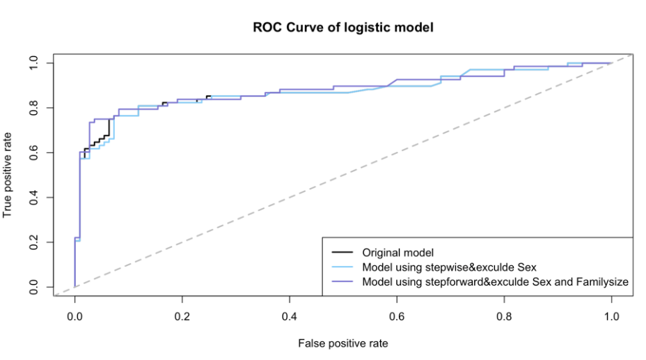
Figure 7: ROC curve of logistic regression
4.2. Decision tree
Default code is used first to run the tree to see how it performed without any interventions (Figure 8). It attains 6 depth and 7 leaf nodes. It chooses the category to split into branches by selecting the best category using the Gini algorithm. Gini is a method for measuring purity in a dataset. Nodes are spilt that maximize the purity within each child node. The accuracy of this model is 80.9%.
Based on these results, maximum depth is changed to 2,3,4,5,6,7 respectively. The model performs better with a higher accuracy when the maximum depth of the tree is 3 (Figure 9). And Gini performs greater than the information gain. It's about 84.83%. In relation to the original one, the branches of this model are cut after Ticket_u, so perhaps the previous tree has the problem of overfitting as the age, embark and fare do not really bring a lot of information. This tree has less calculated time and depth and reduces the model's complexity.
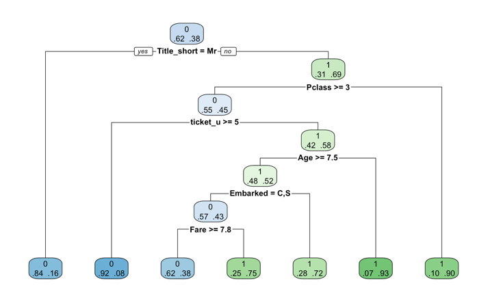
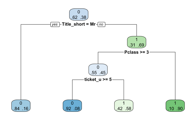
Figure 8: Decision tree (default) | Figure 9: Decision tree with maximum depth 3 |
Table 10: Confusion matrix of decision tree with maximum depth 3
Actual: 0 | Actual: 1 | |
Predicted: 0 | 100 | 10 |
Predicted: 1 | 17 | 51 |
The best complexity parameters (CP) that are tested is 0.001. The depth is 9 and it has a sophisticated classification of the variables (Figure 10). It also has an accuracy of 85.39%. But it needs more calculations as the depth is far deeper. So, this one may be worse at treating very large datasets.
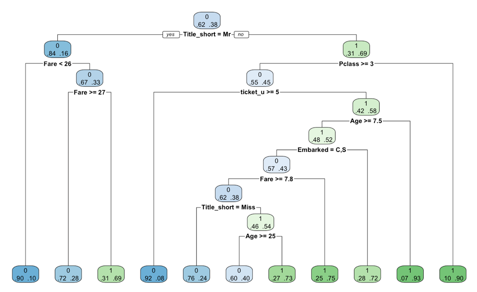
Figure 10: Decision tree with cp 0.001
Table 11: Confusion matrix of decision tree with cp 0.001
Actual: 0 | Actual: 1 | |
Predicted: 0 | 104 | 6 |
Predicted: 1 | 20 | 48 |
4.3. Random forest
Random forests are adopted for less risk of overfitting on decision trees. Regarding choosing the number of trees, the error of the model is plot against the number of trees [6]. The curve almost approaches constant at 200 to 500 trees. Thus, 500 trees are taken and the model gets an accuracy of 83.15%.
Table 12: Confusion matrix of random forest
Actual: 0 | Actual: 1 | |
Predicted: 0 | 99 | 11 |
Predicted: 1 | 19 | 49 |
4.4. Hard voting and final prediction
In conclusion, for the final model, it gets an accuracy of 88%. The sensitivity is 76% and the specificity is 95%. The overall model has more false negatives than false positives. It is better at predicting dead passengers.
Table 13: Confusion matrix of final prediction
Actual:0 | Actual:1 | |
Predicted: 0 | 104 | 16 |
Predicted: 1 | 6 | 52 |
Table 14: Summary of final model
Accuracy | Sensitivity | Specificity | AUC |
0.8764 | 0.7647 | 0.9455 | 0.8932 |
For sub-models, there are more false positives than false negatives. It is better at predicting dead people than surviving passengers. But the overall model, as mentioned above has more false negatives. There are several factors that can be attributed. Initially, there were more dead passengers (439) than survived ones (274) in the training set. So, the models learn more about dead people. Moreover, the variables can represent the characteristics of died passengers than survived such as Sex and Title. For the difference between false positives and false negatives, they may be biased. The sub-models may be similar which will in turn lead to one type of false prediction.
5. Conclusion
This paper builds a model based on the given dataset to predict whether the targets survived or not in the tragedy. According to the hard voting which is based on logistic regression, decision tree and random forest, the model has high accuracy (87.64%) and the voting system is a more objective way to make predictions. Furthermore, decision trees can deal with missing values and the random forest is robust to noise and estimate feature importance which helps to improve the overfitting risk of decision trees. The model can be applied to predicting survival in the navigation field. By the approaches and the process given, enterprises and governments can predict the impact of multiple factors to certain events, which can help them to explore the best way to success.
There are some limitations to the model. In the regression model, the relationship between independent variables and log odds of dependent variables is assumed as linear, although some data may follow a nonlinear relationship. There is still multicollinearity among explanatory variables, affecting accuracy. Improvements can be made through using soft voting which considers the accuracy as weights.
Authors Contribution
All the authors contributed equally and their names were listed in alphabetical order.
References
[1]. Ekinci, E., Omurca, S. İ., & Acun, N. (2018, December). A comparative study on machine learning techniques using Titanic dataset. In 7th international conference on advanced technologies (pp. 411-416).
[2]. Barhoom, A. M., Khalil, A., Abu-Nasser, B. S., Musleh, M. M., & Samy. (2019). Predicting Titanic Survivors using Artificial Neural Network. International Journal of Academic Engineering Research (IJAER), 3(9).
[3]. Exploring Survival on the Titanic. (n.d.). Kaggle.com. https://www.kaggle.com/code/mrisdal/exploring-survival-on-the-titanic
[4]. hiteshp. (2018, September 2). Head Start for Data Scientist. Kaggle.com; Kaggle. https://www.kaggle.com/code/hiteshp/head-start-for-data-scientist#feature-engineering.
[5]. Schreiber-Gregory, Deanna & Bader, Karlen. (2018). Logistic and Linear Regression Assumptions: Violation Recognition and Control.
[6]. thilakshasilva. (2017, December 14). Predicting Titanic Survival using Five Algorithms. Kaggle.com; Kaggle. https://www.kaggle.com/code/thilakshasilva/predicting-titanic-survival-using-five-algorithms#random-forests
[7]. Kraha, A., Turner, H., Nimon, K., Zientek, L. R., & Henson, R. K. (2012). Tools to Support Interpreting Multiple Regression in the Face of Multicollinearity. Frontiers in Psychology, 3. https://doi.org/10.3389/fpsyg.2012.00044
[8]. Mohr, D. L., Wilson, W. J., & Freund, R. J. (2022, January 1). Chapter 7 - Linear Regression (D. L. Mohr, W. J. Wilson, & R. J. Freund, Eds.). ScienceDirect; Academic Press. https://www.sciencedirect.com/science/article/abs/pii/B9780128230435000072
[9]. Song, Y. Y., & Lu, Y. (2015). Decision tree methods: applications for classification and prediction. Shanghai archives of psychiatry, 27(2), 130–135. https://doi.org/10.11919/j.issn.1002-0829.215044
[10]. Speiser, J. L., Miller, M. E., Tooze, J., & Ip, E. (2019). A Comparison of Random Forest Variable Selection Methods for Classification Prediction Modeling. Expert Systems with Applications, 134(1), 93–101. https://doi.org/10.1016/j.eswa.2019.05.028
[11]. Shareef, A.Q., Kurnaz, S. Deep Learning Based COVID-19 Detection via Hard Voting Ensemble Method. Wireless Pers Commun (2023). https://doi.org/10.1007/s11277-023-10485-2
Cite this article
Liao,Y.;Zhang,S.;Zhang,Z. (2025). Research on Titanic Survival Prediction Based on Machine Learning Method. Advances in Economics, Management and Political Sciences,152,152-162.
Data availability
The datasets used and/or analyzed during the current study will be available from the authors upon reasonable request.
Disclaimer/Publisher's Note
The statements, opinions and data contained in all publications are solely those of the individual author(s) and contributor(s) and not of EWA Publishing and/or the editor(s). EWA Publishing and/or the editor(s) disclaim responsibility for any injury to people or property resulting from any ideas, methods, instructions or products referred to in the content.
About volume
Volume title: Proceedings of the 3rd International Conference on Financial Technology and Business Analysis
© 2024 by the author(s). Licensee EWA Publishing, Oxford, UK. This article is an open access article distributed under the terms and
conditions of the Creative Commons Attribution (CC BY) license. Authors who
publish this series agree to the following terms:
1. Authors retain copyright and grant the series right of first publication with the work simultaneously licensed under a Creative Commons
Attribution License that allows others to share the work with an acknowledgment of the work's authorship and initial publication in this
series.
2. Authors are able to enter into separate, additional contractual arrangements for the non-exclusive distribution of the series's published
version of the work (e.g., post it to an institutional repository or publish it in a book), with an acknowledgment of its initial
publication in this series.
3. Authors are permitted and encouraged to post their work online (e.g., in institutional repositories or on their website) prior to and
during the submission process, as it can lead to productive exchanges, as well as earlier and greater citation of published work (See
Open access policy for details).
References
[1]. Ekinci, E., Omurca, S. İ., & Acun, N. (2018, December). A comparative study on machine learning techniques using Titanic dataset. In 7th international conference on advanced technologies (pp. 411-416).
[2]. Barhoom, A. M., Khalil, A., Abu-Nasser, B. S., Musleh, M. M., & Samy. (2019). Predicting Titanic Survivors using Artificial Neural Network. International Journal of Academic Engineering Research (IJAER), 3(9).
[3]. Exploring Survival on the Titanic. (n.d.). Kaggle.com. https://www.kaggle.com/code/mrisdal/exploring-survival-on-the-titanic
[4]. hiteshp. (2018, September 2). Head Start for Data Scientist. Kaggle.com; Kaggle. https://www.kaggle.com/code/hiteshp/head-start-for-data-scientist#feature-engineering.
[5]. Schreiber-Gregory, Deanna & Bader, Karlen. (2018). Logistic and Linear Regression Assumptions: Violation Recognition and Control.
[6]. thilakshasilva. (2017, December 14). Predicting Titanic Survival using Five Algorithms. Kaggle.com; Kaggle. https://www.kaggle.com/code/thilakshasilva/predicting-titanic-survival-using-five-algorithms#random-forests
[7]. Kraha, A., Turner, H., Nimon, K., Zientek, L. R., & Henson, R. K. (2012). Tools to Support Interpreting Multiple Regression in the Face of Multicollinearity. Frontiers in Psychology, 3. https://doi.org/10.3389/fpsyg.2012.00044
[8]. Mohr, D. L., Wilson, W. J., & Freund, R. J. (2022, January 1). Chapter 7 - Linear Regression (D. L. Mohr, W. J. Wilson, & R. J. Freund, Eds.). ScienceDirect; Academic Press. https://www.sciencedirect.com/science/article/abs/pii/B9780128230435000072
[9]. Song, Y. Y., & Lu, Y. (2015). Decision tree methods: applications for classification and prediction. Shanghai archives of psychiatry, 27(2), 130–135. https://doi.org/10.11919/j.issn.1002-0829.215044
[10]. Speiser, J. L., Miller, M. E., Tooze, J., & Ip, E. (2019). A Comparison of Random Forest Variable Selection Methods for Classification Prediction Modeling. Expert Systems with Applications, 134(1), 93–101. https://doi.org/10.1016/j.eswa.2019.05.028
[11]. Shareef, A.Q., Kurnaz, S. Deep Learning Based COVID-19 Detection via Hard Voting Ensemble Method. Wireless Pers Commun (2023). https://doi.org/10.1007/s11277-023-10485-2