1. Introduction

The first letters of the three words gold, black gold, and US dollars just form the God worshipped by Christianity. The world's financial and economic pursuit of gold, black gold, and US dollars is just like the worship of God by Christians. The reason why gold is respected by people is that it is determined by the nature of gold itself. As a precious metal, gold has excellent physical properties and stable chemical properties, and is widely used in various fields. On the other hand, gold has excellent hedging function and the gold market is difficult to control, so gold has strong investment benefits. Throughout the ages, gold has been used by people to preserve wealth. In August 2015, stock markets around the world took a hit, with stock prices plummeting, with the S&P 500 down 10%, but the dollar-denominated gold price up 5%. This phenomenon also occurred in the "Black Monday" of 1987 and the financial crisis in 2007. There are many more examples of how gold's value continues to rise every year during times of war and economic downturns. In recent years, as an investment product, gold has attracted more and more attention. The price of gold has also become the focus of people. With the increasing role of the gold market, statistics and forecasts on the fluctuations and prices of the gold market have attracted widespread attention. Zou believes that in the long run, holding gold can effectively diversify the risk of bond market and inflation [1]. Analysis by the World Gold Council shows that during market volatility, gold can be used in investment portfolios to protect global purchasing power [2]. Gold is currently becoming a scarce resource. Because the value effect of prospecting has dropped by 40% compared with previous years. The latest report from the World Gold Council shows that central banks continue to buy gold [3].

So far, scholars in various fields have found that the fluctuations of the gold market are not irregular, but have certain predictability through their research on the gold market. Through the establishment of various models to conduct research on gold price prediction, a number of theoretical research results have been obtained. Xie et al. used the M-Copula-GJR-VaR model to effectively improve the hedging effect and asset returns [4]. Chen et al. analyzed the relevant factors that affect the price of gold [5]. Using the organic combination of neural network model and ARMA, the prediction of gold price is realized. And gives some trading suggestions for gold-related derivatives. Cao constructed a timing trading strategy after optimizing the penalty parameters in the SVM model and the parameters in the kernel function with the goal of minimizing MSE [6]. Cheng used the grey correlation degree to analyze the factors that significantly affect the price of gold, and established a multi-factor BP neural network model. The economic factors that significantly affect the price of gold are added to the forecast model, which improves the forecast accuracy [7]. Xu made a statistical analysis of the closing price of the Shanghai Gold Exchange on the last trading day of each month. A quadratic curve fitting model is established and short-term prediction is made based on it, which provides a reference for investors to invest in gold [8]. Wang used a variable coefficient regression model to predict the gold price, which greatly improved the prediction accuracy [9]. The dynamic evolution of gold prices reflects the investment decisions of economic actors in the financial market. The dynamic evolution process of gold price is also a process of data generation [10]. There are many methods used by domestic and foreign scholars to study the trend of gold price. But it has certain limitations. This paper used the time series correlation theory to establish an ARIMA model for the gold price in the London gold exchange market. and conduct empirical analysis.

In the eyes of many investors, gold is a "veritable" value preservation and appreciation product. Statistics show that over the past 12 years, the price of gold has risen continuously from nearly $300 to nearly $1,900 per ounce. However, with the large fluctuations in market prices, the risk of blindly purchasing gold to preserve and increase its value cannot be ignored [11]. Yin and others pointed out that the correlation between the gold spot and the average futures return and other factors changes with time, positive correlation and negative correlation appear alternately, and the time-varying is obvious. Whether it can be used as a safe-haven asset in the real economy or the stock market varies from time to time [12]. Therefore, in-depth research on the price of gold can allow us to better predict the price of gold. It not only helps the country to adjust economic policies in a timely manner, but also helps individuals and institutions to control financial risks. It has theoretical and applied value.

2. Methodology

The goal of this article is to analyze the gold price fluctuations and trends in 2018 based on the ARIMA model. By fitting and evaluating the corresponding models, the ideas and methods of modeling are shown in the figure 1, the following are detailed explanation.

After the data is collected, the data for 2018 is preprocessed. Through the test of the time series chart, it is observed that the data has no periodicity and has a clear downward trend. After the unit root test, a P value greater than 0.05 was obtained. It shows that the series is non-stationary, so the time series data needs to be differentiated. After the first difference, a stationary series is obtained. The white noise test shows that the P value is less than 0.05 at the 6th and 12th order delays. Prove that the sequence is a non-white noise sequence. Then proceed to follow-up experiments.

Plot autocorrelation plots and partial autocorrelation plots of the model, as well as the results of automatic ordering of the model. Comparing the AIC values of ARIMA (1,2,1), ARIMA (2,2,2), ARIMA (3,2,3) and other related models, comprehensive test conditions and prediction effects, the most ideal model for the sequence should be ARIMA (2,2,2) model. Based on the conditional least squares estimation method, the fitting results of the ARIMA (2,2,2) model are obtained as follows: \( {∇^{2}}{x_{t}}=\frac{1-0.925B+0.929{B^{2}}}{1-0.998B-0.174{B^{2}}}{ε_{t}}\ \ \ (1) \)

After the ideal model is obtained, the model and parameters are tested for significance. It is obtained that the P value is greater than 0.05 at the 6th and 12th order delays. Therefore, the null hypothesis is not rejected. This shows that all model-related information has been extracted, and the sequence is a purely random sequence. It is proved that the residual sequence of the fitted model belongs to the white noise sequence, that is, the fitted model is significantly effective. By constructing t-statistics, it was found that at a significance level of 0.05, the P-values for all parameters were less than 0.05. Therefore, the null hypothesis that the parameter is significantly 0 is rejected, that is, the parameter significance test of the model is passed.

After the model passes the test. By comparing with the future real value, it can be obtained that the prediction result of the corresponding model in the next 5 days is better. It has a good reference value for investors.

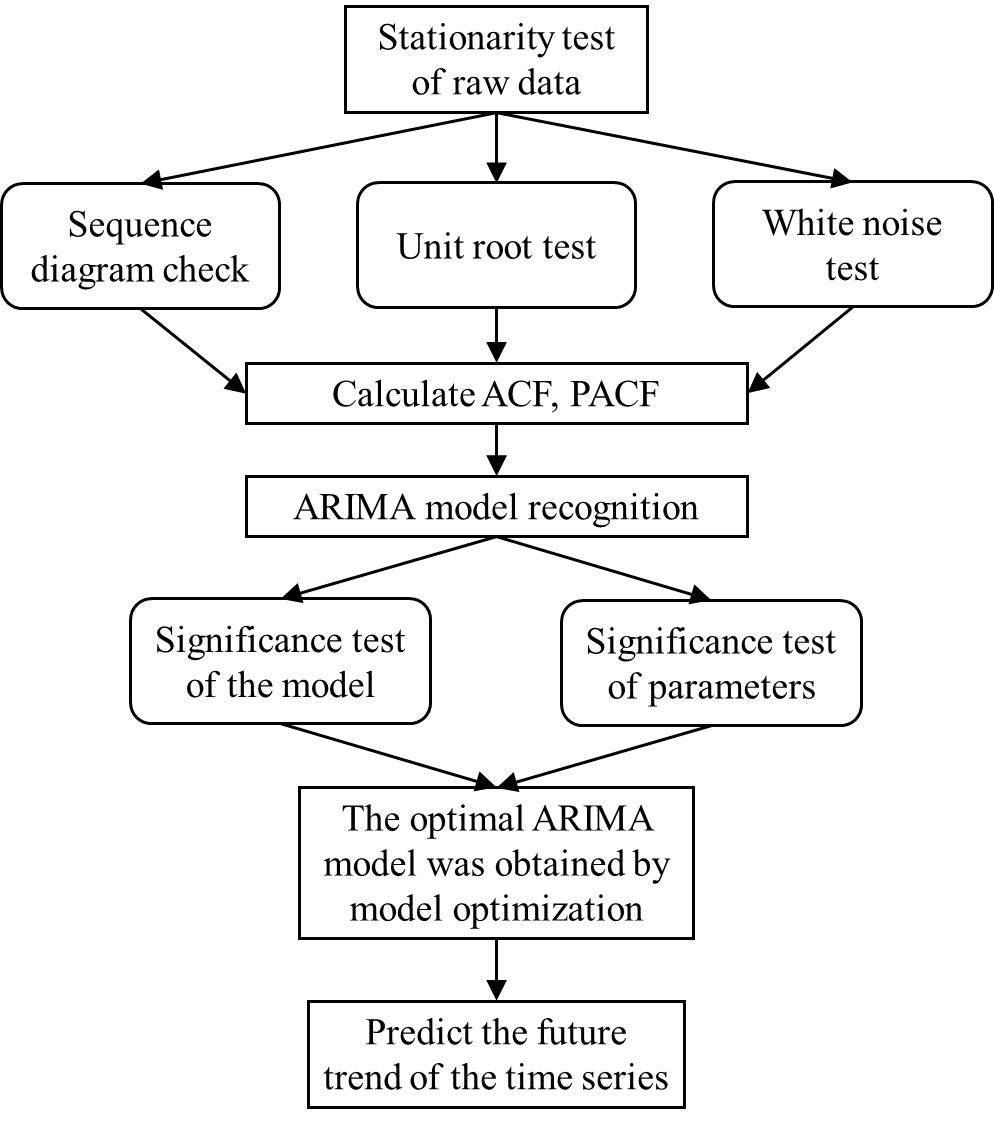
Figure 1. Frame diagram of paper.

3. Results and discussion

The following section selects the data from 2018.1.18–2018.7.18. Based on the final transaction amount on normal trading days, there are a total of 126 sample data. Analyze and compare the establishment of ARIMA (2,2,2) model, and predict the future trend of gold.

3.1. Pre-processing of raw data

3.1.1. Sequence diagram check. The timing diagram inspection mainly refers to the inspection method that makes judgments according to the characteristics of the timing diagram. Graph tests of stationarity rely on the principle that stationary time series have constant mean and variance. This means that a log series test plot for a stationary series should show that the series fluctuates consistently around a constant value, and the fluctuation range is bounded.

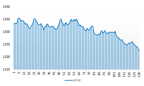
Figure 2. Time series chart of gold price movements.

From the time series plot (Figure 2), there is a clear downward trend in the data. The series does not appear to fluctuate consistently around a constant value, and the fluctuations are not periodic. Therefore, it is preliminarily judged that the data is not stable.

3.1.2. Unit root (ADF) test. The unit root test (ADF test) is the most common method for constructing a statistic for stationarity testing. In order to accurately judge whether the original series is stationary, it is necessary to further perform unit root test on the data. As shown in the table below. p=0.803, greater than 0.05, it is concluded that the series is non-stationary. The data needs to be differentially processed.

Table 1. ADF test of raw data.

3.1.3. Sequence diagram after second order difference. The series has a clear downward trend before the difference, so the series is not stationary. It can be seen from Figure 3 that after the difference, it can be clearly seen that the sequence has no obvious trend. It fluctuates up and down within a certain constant range, so it can be preliminarily judged that the sequence is stable. Then proceed to the following experiment.

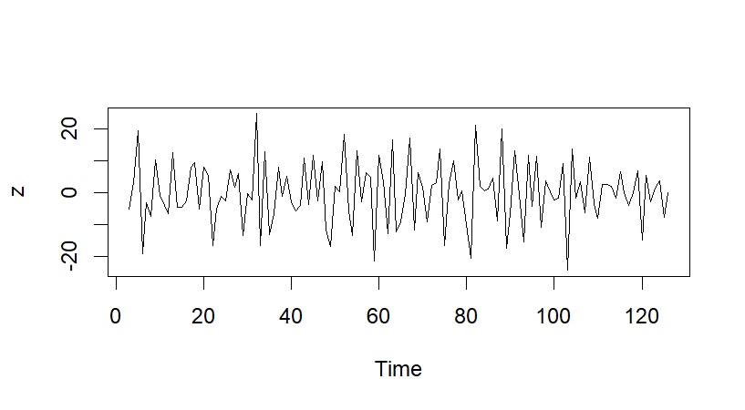
Figure 3. Sequence diagram after second order difference.

3.1.4. Unit root (ADF) test after difference. As shown in the table below, it can be seen from the results of the ADF test after the difference. P<0.01, less than the significant level of α of 0.05, it can be considered that the series is a stationary series after the second-order difference. In order to facilitate subsequent pure randomness testing. If the sequence is stationary, the situation will be simpler. Well-established stationary series modelling methods can be used.

Table 2. ADF test after difference.

3.1.5. White noise test. In order to ensure the validity of the subsequent experiments, the white noise test is carried out on the time series. As shown in the table below, it is found that the P values corresponding to the LB statistic are all less than the significant level ( \( α \) =0.05) after the 6th-order delay and the 12th-order delay. Therefore, the null hypothesis that the sequence is a random sequence (the null hypothesis is white noise) is rejected, and the sequence is considered to be a non-white noise sequence.

Table 3. White noise test.

3.2. Model identification

3.2.1. Order determination and discrimination of models. The following are the autocorrelation diagram (Fig. 4) and the partial autocorrelation diagram (Fig. 5) after the second order difference of the sequence. The model is automatically ordered.

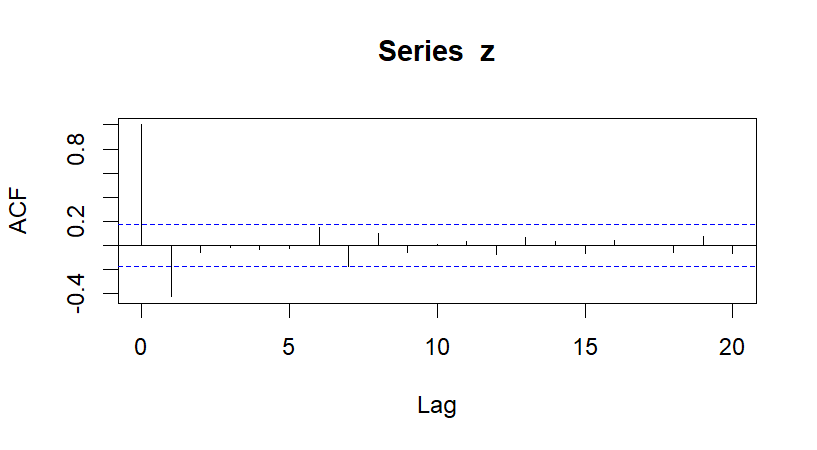
Figure 4. Since the correlation diagram.

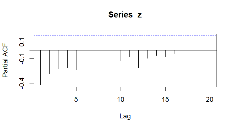
Figure 5. Partial autocorrelation graph.

Compare the AIC values of related models such as MA (1), AR (2), ARIMA (1,2,1), ARIMA (2,2,2), ARIMA (3,2,3). According to the comprehensive test situation and prediction results, the most ideal model for obtaining the sequence should be the ARIMA (2,2,2) model.

Table 4. Parameter estimation.

ARIMA(p, d, q) model:

\( Φ(B){∇^{d}}{x_{t}}=Θ(B){ε_{t}}\ \ \ (2) \)

\( E({ε_{t}})=0\ \ \ (3) \)

\( Var({ε_{t}})=σ_{ε}^{2}\ \ \ (4) \)

\( E({ε_{t}}{ε_{s}})=0  s≠t \ \ \ (5) \)

\( E({x_{s}}{ε_{t}})=0 ∀s \lt t\ \ \ (6) \)

\( Φ(B) \) is the delay operator acting on the error sequence； \( {∇^{d}} \) is \( d \) -order difference sequence； \( {x_{t}} \) is a sequence value at time t； \( Θ(B) \) is the delay operator acting on \( {x_{t}} \) ； \( {ε_{t}} \) is the error of \( t \) time； \( {ε_{s}} \) is the error of \( s \) time； \( {x_{s}} \) is a sequence value at time \( s \) ； \( σ_{ε}^{2} \) represents the variance of \( ε \) ； \( B \) is a form of the delay operator； \( E({ε_{t}}{ε_{s}}) \) is the product of the expected value of \( {ε_{t}} \) and \( {ε_{s}} \) , indicating that the errors at different times are irrelevant; \( E({x_{s}}{ε_{t}}) \) is the product of \( {x_{s}} \) and \( {ε_{t}} \) expected value.

To sum up, based on the conditional least squares estimation method, the fitting result is obtained as:

\( {∇^{2}}{x_{t}}=\frac{1-0.925B+0.929{B^{2}}}{1-0.998B-0.174{B^{2}}}{ε_{t}}\ \ \ (7) \)

3.2.2. Significance test of ARIMA (2,2,2) model. By performing a white noise test. As shown in the table below, it can be concluded that the ARIMA (2,2,2) model has p-values significantly greater than 0.05 at delays 6 and 12. Therefore, the null hypothesis is not rejected. Indicates that model-related information has been extracted. The sequence is a purely random sequence. It is proved that the residual sequence of the fitted model belongs to the white noise sequence, that is, the fitted model is significantly effective.

Table 5. Significance test of the model.

3.2.3. Significance test of parameters. The T statistic was constructed and parametric test was performed, and the results were as follows:

Table 6. Significance test of parameters.

The T statistic is being constructed as shown in the table. The significance level is at 0.05. The P value for \( {T_{1}} \) is less than 0.05, rejecting the null hypothesis that the parameter is significantly 0. The P value for \( {T_{2}} \) is less than 0.05, rejecting the null hypothesis that the parameter is significantly 0. The P value corresponding to \( {T_{3}} \) is less than 0.05, rejecting the null hypothesis that the parameter is significantly 0. The P value corresponding to \( {T_{4}} \) is less than 0.05, rejecting the null hypothesis that the parameter is significantly 0. Therefore, the parametric significance test of the model is passed.

3.3. Model to predict

After the previous data preprocessing and the significance test of the model and parameters. The model can be further used to predict the future trend of the series, as shown in the figure below.

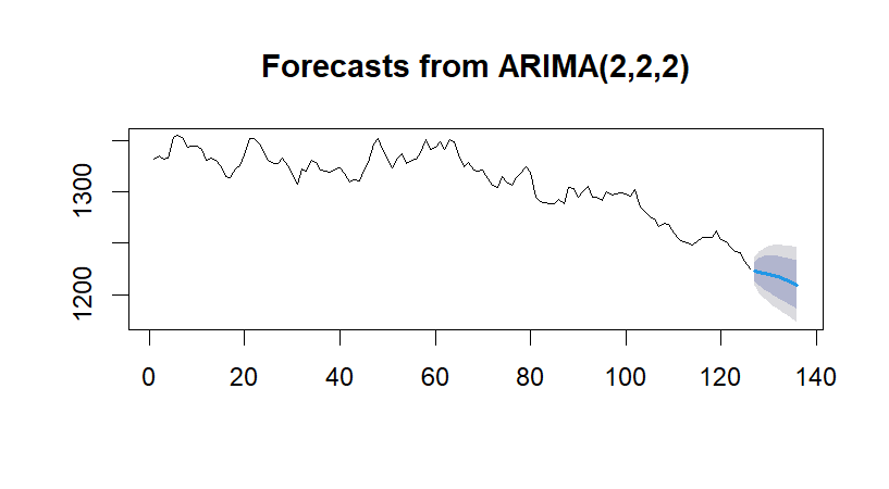
Figure 6. Sequence prediction graph.

The image above shows the forecast for this time series. It can be seen from the chart that the price of gold is still in a downward trend in the next 5 days. The tested ARIMA (2,2,2) model was used for fitting. It can more accurately predict the price of gold for many days in the future. Here is an example of the price of gold for the next five days, as shown in the table below.

Table 7. Predicted value and confidence interval.

By comparing the predicted value with the actual value, it is found that there is little difference between the two. The ARIMA (2,2,2) model has good prediction results and can be used to predict the price fluctuation of the US dollar against gold. The forecast has a good reference significance for the formulation of corresponding national economic policies.

4. Conclusion

This paper conducts an empirical analysis of the gold price data in 2018 based on the ARIMA model. After the time series test and the unit root test, it is known that the daily price of gold is a non-stationary sequence. Then, a stationary sequence is obtained by differential processing, and the sequence is determined as a non-white noise sequence by white noise test. Finally, by comparing the AIC values of different ARIMA models, the optimal time series model ARIMA (2,2,2) is obtained. After this, the gold price forecast for the next five days is made and the result is better. This has good guiding significance for investors and the market.

Since this article selects 6 months of data in 2018 for analysis, it estimates the price trend of gold in the short term. Therefore, it is impossible to give a good forecast for the price of gold in the long term. For short-term data operations, the impact of the long-term memory of financial assets (historical events will affect the price of financial assets for a long time) can be ignored, providing a reference for short-term investors. To predict the trend of gold prices more accurately, long-term influencing factors cannot be ignored. Further research in this direction can be carried out in the future.

References

[1]. Zou Q 2014 Research on the Financial Function of Gold (Shanghai: Shanghai Academy of Social Sciences)
[2]. Duan H 2021 Research on Gold Futures Price Prediction Based on Time Series (Harbin: Harbin Institute of Technology)
[3]. Ou H 2016 Statistical Analysis and Prediction of Gold Price (Fijian: Fujian Normal University).
[4]. Xie C, Qu M and Wang G 2013 Study on the Optimal Hedging Ratio of Gold Market Based on M-Copula-GJR-VAR Model (Management science) 26(02) pp 90-99
[5]. Chen X, Tian L and Han X 2018 Gold price forecast analysis and research. Journal of Foshan University of Science and Technology (Natural Science Edition) 36(04) pp 6-10
[6]. Cao X 2017 Gold Price Prediction Model and Parameter Optimization Based on SVM (Shandong: Shandong University)
[7]. Cheng M 2020 Research on Forecasting Method of International Gold Price (Shandong: Shandong University)
[8]. Chen Xu 2015 Application of Time Series in Gold Price Forecasting Business 2015(16) pp 180-181
[9]. Wang Y 2010 Research on Gold Price Forecast Based on Variable Coefficient Regression Model (Tianjin: Tianjin University)
[10]. Pan X 2020 Empirical Analysis of Gold Price Based on ARIMA-GARCH Model Business 2020 (20) pp 155-156
[11]. Chen Y 2013 Can Gold Hold its Value with Volatile Prices? NCNA 2013-05-03(006)
[12]. Yin L and Liu Y 2015 Is Gold a Stable Haven? —— From the Perspective of Macroeconomic Uncertainty International Financial Studies 2015(07) pp 87-96
Cite this article
Gao,D.L.;Liang,J.Y.;Xu,B.H. (2023). Predict Gold Price Trend Based on ARIMA Model. Theoretical and Natural Science,2,157-165.
Data availability
The datasets used and/or analyzed during the current study will be available from the authors upon reasonable request.
Disclaimer/Publisher's Note
The statements, opinions and data contained in all publications are solely those of the individual author(s) and contributor(s) and not of EWA Publishing and/or the editor(s). EWA Publishing and/or the editor(s) disclaim responsibility for any injury to people or property resulting from any ideas, methods, instructions or products referred to in the content.
About volume
Volume title: Proceedings of the International Conference on Computing Innovation and Applied Physics (CONF-CIAP 2022)
© 2024 by the author(s). Licensee EWA Publishing, Oxford, UK. This article is an open access article distributed under the terms and
conditions of the Creative Commons Attribution (CC BY) license. Authors who
publish this series agree to the following terms:
1. Authors retain copyright and grant the series right of first publication with the work simultaneously licensed under a Creative Commons
Attribution License that allows others to share the work with an acknowledgment of the work's authorship and initial publication in this
series.
2. Authors are able to enter into separate, additional contractual arrangements for the non-exclusive distribution of the series's published
version of the work (e.g., post it to an institutional repository or publish it in a book), with an acknowledgment of its initial
publication in this series.
3. Authors are permitted and encouraged to post their work online (e.g., in institutional repositories or on their website) prior to and
during the submission process, as it can lead to productive exchanges, as well as earlier and greater citation of published work (See
Open access policy for details).