1. Introduction

In the context of globalization, exchange rate, as part of the core variables in international economic exchanges, directly affects international trade, capital flows, and the economic policies of various countries [1]. Exchange rate is not only the conversion ratio between currencies but also an important manifestation of a country's economic health and international competitiveness. Meanwhile, gross domestic product (GDP), as a key indicator for measuring a country's economic scale and growth level, reflects the total volume of economic activities within a certain period. The relationship between GDP and exchange rate is not only an important topic in macroeconomic research but also a focus for governments and international investors. Therefore, studying the relationship between exchange rates and GDP is becoming more and more important in the 21st century [2].

In recent years, many researchers studied the relationship between exchange rates and GDP from various perspectives. The most typical one is to study the effect of exchange rate fluctuations on GDP, especially in developing countries. Many researchers found that the relationship between exchange rate and GDP growth is non-linear. Moderate exchange rate fluctuations have a positive impact on economic growth, but excessive fluctuations will restrain economic growth. Moreover, the influence of exchange rate on GDP shows significant differences in developing countries and developed countries. Exchange rate depreciation has played an essential role on the GDP growth of developing countries, but has a relatively minor effect on developed countries [3]. Most of the studies used panel data regression analysis and VAR model. Although there are multiple aspects toward the research of exchange rates and GDP, only a few researchers focus on certain countries. More researchers focus on macroscopic research and ignore the differences of the impact of exchange rates in different countries. Therefore, this study focuses on 3 countries and analyzes the relationships between exchange rates and GDP, aiming to understand the impact of exchange rates under different economic systems.

The study consists of 4 parts. The first one is introduction, which includes the summary of recent studies in exchange rates and GDP and the conclusion of those studies. The second one is the method and theory used in this study, which involves linear regression and locally weighted regression. The third one is results and discussion, in which the author discusses the causes of the results. The last one is conclusion, involving the prospect of further study and the limitations of current study.

2. Method and Theory

2.1. Linear Regression

The author uses linear regression and locally weighted regression to find the best fit. The basic formulas are shown below. Simple linear regression is a technique that is often employed to examine the complex interplay of two variables, \( Y \) and \( X \) . Suppose that there is a value of \( X \) , denoted as \( X \) = \( x \) , is provided, it becomes possible to calculate the corresponding data point of \( Y \) . Most mathematicians define that the regression of a random variable \( Y \) on the other variable \( X \) is \( E(Y|X=x), \) which shows the predicted measure of \( Y \) when \( X \) = \( x \) [4]. If the regression of \( Y \) on \( X \) is linear, it can be found that

\( E{(Y∣X=x)}={β_{0}}+{β_{1}}x\ \ \ (1) \)

where the unknown parameters \( {β_{0}} \) represents the intercept, and \( {β_{1}} \) determines the slope of a certain fitted equation. Suppose \( {Y_{1}} \) , \( {Y_{2}} \) , …, \( {Y_{n}} \) are independent observations of the random variable \( Y \) , recorded at the values \( {x_{1}} \) , \( {x_{2}} \) , …, \( {x_{n}} \) of a random variable \( X \) . If the regression of \( Y \) on \( X \) is linear, then for each \( i=1,2,……n \)

\( {Y_{i}}=E{(Y∣X=x)}+{e_{i}}={β_{0}}+{β_{1}}x+{e_{i}}\ \ \ (2) \)

The term \( {e_{i}} \) accounts for random error, which arises due to unpredictable variations in \( Y \) that cannot be explained by \( X \) . This random error is independent of \( x \) and does not convey any information about \( Y \) (if it did, it would be considered a systematic error).

To proceed, one needs to predict the population slope and intercept. In practice, one usually works with a sample of data rather than the entire data set. Since the population slope \( {β_{1}} \) and intercept \( {β_{0}} \) are unable to be known, they must be estimated from the sample data. This can be accomplished through determining the line that best fits the population data, whose \( {β_{0}} \) and \( {β_{1}} \) can make \( {\hat{y}_{i}}={b_{0}}+{b_{1}}{x_{i}} \) the closest among all the \( {\hat{y}_{i}} \) to \( {y_{i}} \) [5].

In realization, the author wishes to minimize the discrepancy between the observed value of \( y \) ( \( {y_{i}} \) ) and its predicted counterpart \( y \) ( \( {\hat{y}_{i}} \) ). This difference is termed the residual, denoted as \( {\hat{e}_{i}} \) , and is calculated as:

\( {\hat{e}_{i}}={y_{i}}-{\hat{y}_{i}}\ \ \ (3) \)

A widely-used approach for selecting \( {β_{0}} \) and \( {β_{1}} \) is the least squares method. This method aims to minimize the total of squared residuals, also known as the residual sum of squares [ \( RSS \) ],

\( RSS=\sum _{i=1}^{n}\hat{e}_{i}^{2}=\sum _{i=1}^{n}{({y_{i}}-{\hat{y}_{i}})^{2}}=\sum _{i=1}^{n}{({y_{i}}-{b_{0}}-{b_{1}}{x_{i}})^{2}} \ \ \ (4) \)

To ensure \( RSS \) is minimized with respect to \( {b_{0}} \) and \( {b_{1}} \) , the following conditions must be met:

\( \frac{∂RSS}{∂{b_{0}}}=-2\sum _{i=1}^{n} ({y_{i}}-{b_{0}}-{b_{1}}{x_{i}})=0\ \ \ (5) \)

By rearranging the order of the terms in the last two equations, it is found that

\( \sum _{i=1}^{n} {y_{i}}={b_{0}}n+{b_{1}}\sum _{i=1}^{n} {x_{i}}\ \ \ (6) \)

\( \sum _{i=1}^{n} {x_{i}}{y_{i}}={b_{0}}\sum _{i=1}^{n} {x_{i}}+{b_{1}}\sum _{i=1}^{n} x_{i}^{2}\ \ \ (7) \)

The above equations are referred to as the normal equations. By solving them simultaneously, people may achieve the least squares estimates for the intercept

\( {\hat{β}_{0}}=\overline{y}-{\hat{β}_{1}}\overline{x}\ \ \ (8) \)

The slope is given by

\( {\hat{β}_{1}}=\frac{\sum _{i=1}^{n}{x_{i}}{y_{i}}-n\overline{xy}}{\sum _{i=1}^{n}x_{i}^{2}-n{\overline{x}^{2}}}=\frac{\sum _{i=1}^{n}({x_{i}}-\overline{x})({y_{i}}-\overline{y})}{\sum _{i=1}^{n}{({x_{i}}-\overline{x})^{2}}}=\frac{SXY}{SXX}\ \ \ (9) \)

2.2. Locally Weighted Regression

A majority of linear regression forms can be remolded into a “double representation” where the prediction values are based not only on linear regression but also on linear combinations of a kernel function computed at training data points. This approach is particularly relevant for models that rely on a predefined nonlinear feature space mapping \( ϕ(x) \) , where the kernel function can be defined as:

\( k(x,{x^{ \prime }})=ϕ{(x)^{T}}ϕ({x^{ \prime }})\ \ \ (10) \)

According to the perspective above, the author concludes that the kernel function demonstrates symmetry concerning its arguments:

\( k(x, {x^{ \prime }})= k({x^{ \prime }}, x).\ \ \ (11) \)

By defining a kernel as an inner product in a feature space, the kernel trick (or kernel substitution) allows for the expansion of multiple algorithms [5]. The main idea is that if an algorithm's input vector \( x \) is only involved in scalar products, these products can be exchanged with different kernel functions.

Here, one considers a linear regression model of which parameters are determined by minimizing a regularized sum-of-squares error function given by

\( J(w)=\frac{1}{2}\sum _{n=1}^{N}{\lbrace {w^{T}}ϕ({x_{n}})-{t_{n}}\rbrace ^{2}}+\frac{λ}{2}{w^{T}}w \ \ \ (12) \)

in which \( λ \) \( ≥0 \) . Let the gradient of \( J(w) \) with vanishing \( w \) , the equation for \( w \) takes the form of a linear integration of the vectors \( ϕ({x_{n}}) \) with coefficients dependent on \( w \) :

\( w=-\frac{1}{λ}\sum _{n=1}^{N}\lbrace {w^{T}}ϕ({x_{n}})-{t_{n}}\rbrace ϕ({x_{n}})=\sum _{n=1}^{N}{a_{n}}ϕ({x_{n}})={Φ^{T}}a\ \ \ (13) \)

In the formula, \( Φ \) represents the design matrix, with the \( n th \) row provided by \( {ϕ({x_{n}})^{T}} \) .The vector \( a={(\begin{matrix}{a_{1}},…,{a_{N}} \\ \end{matrix})^{T}} \) ,and the author has framed:

\( {a_{n}}=-\frac{1}{λ}\lbrace {w^{T}}ϕ({x_{n}})-{t_{n}}\rbrace \ \ \ (14) \)

The least-squares algorithm can be reformulated from the perspective of the parameter vector \( a \) rather than calculating with \( w \) [6]. Substituting \( w = {Φ^{T}}a \) into \( J(w) \) yields:

\( J(a)=\frac{1}{2}{a^{T}}Φ{Φ^{T}}Φ{Φ^{T}}a-{a^{T}}Φ{Φ^{T}}t+\frac{1}{2}{t^{T}}t+\frac{λ}{2}{a^{T}}Φ{Φ^{T}}a\ \ \ (15) \)

Here, \( t={({t_{1}},…,{t_{N}})^{T}} \) .Now it can be defined that the Gram matrix \( K= \) \( Φ{Φ^{T}} \) ,which is an N \( × \) N symmetric matrix with elements

\( {K_{nm}}=ϕ{({x_{n}})^{T}}ϕ({x_{m}})=k({x_{n}},{x_{m}})\ \ \ (16) \)

The kernel function \( k(x,{x^{ \prime }}) \) is characterized as in (10). The sum-of-squares error function can be expressed in terms of the Gram matrix as

\( J(a)=\frac{1}{2}{a^{T}}KKa-{a^{T}}Kt+\frac{1}{2}{t^{T}}t+\frac{λ}{2}{a^{T}}Ka\ \ \ (17) \)

Set the gradients of \( J(a) \) regarding \( a \) to zero, the author obtained the answer:

\( a={(K+λ{I_{N}})^{-1}}t\ \ \ (18) \)

When it is reinserted into the linear regression, one can get the prediction value for a new input \( x \)

\( y(x)={w^{T}}ϕ(x)={a^{T}}Φϕ(x)=k{(x)^{T}}{(K+λ{I_{N}})^{-1}}t\ \ \ (19) \)

This dual formulation demonstrates that the outcome to the least-squares problem can be depicted totally using the kernel function \( k(x, x \prime ) \) .

3. Results and Discussion

3.1. Linear Regression of Exchange Rates

In this section, the author chooses 3 countries in Asia to study the relationship between their exchange rates and GDP. The 3 countries are South Korea, Japan and Singapore [7]. There are multiple reasons for choosing these 3 countries. To begin with, the economic structure of the three countries has its own characteristics. Japan is a highly industrialized country, South Korea is a newly industrialized country, and Singapore is a city-state dominated by services and finance. This diversity is helpful to analyze the correlation between exchange rate and GDP under different economic structures. Moreover, the exchange rate policies that have been carried out in these 3 countries are quite different. Japan and South Korea have floating exchange rate systems, while Singapore has a managed floating exchange rate system. These different exchange rate policies provide rich cases for studying the impact of exchange rate changes on GDP. In addition, South Korea, Japan and Singapore are all highly open economies, with international trade and investment playing an important role in their economies. This makes the impact of exchange rate changes on GDP more significant, which is suitable for studying the relationship between exchange rate and GDP.

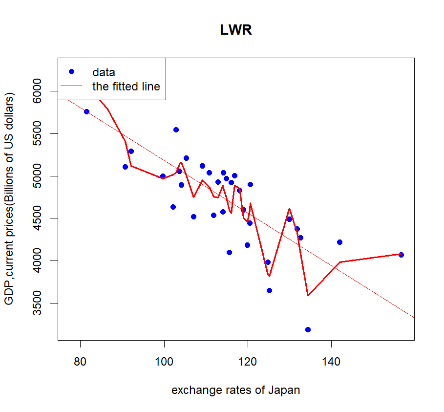
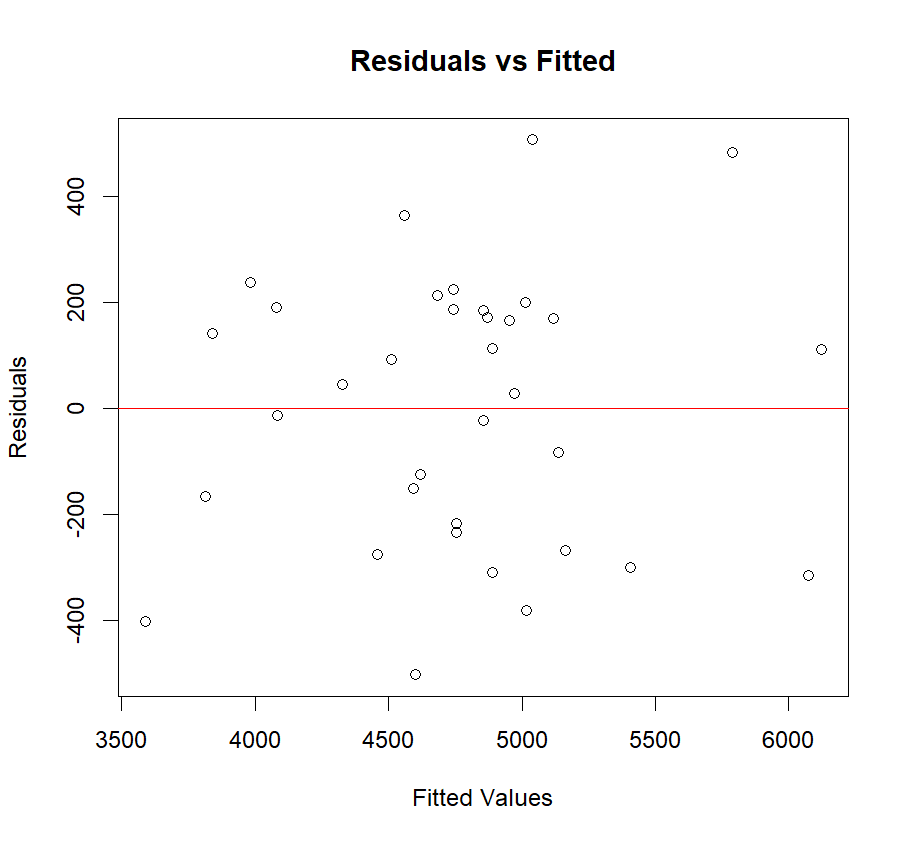
Figure 1: Left: the LWR and linear regression of exchange rates and GDP in Japan; Right: the residuals versus the fitted values.

Therefore, the author searched for the data of their exchange rates and GDP from 1990 to 2024 of those three countries then use them as the data sets of this study. Based on the basic theory of linear regression and locally weighted regression, the author utilizes these regression models to achieve a better fit for the three data sets. The results are as follows.

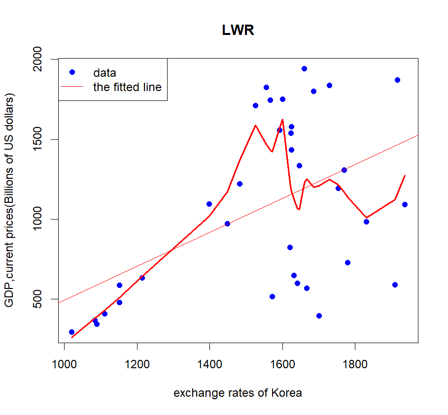
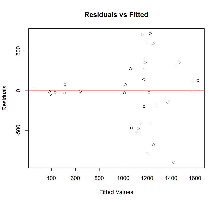
Figure 2: Left: the LWR and linear regression of exchange rates and GDP in South Korea; Right: the residuals versus the fitted values. The best span for South Korea is 0.35.

The author uses cross-validation to find the best span for the LWR, which enables the MSE to be the smallest. The dataset is segmented by the author into a training set and a test set. For every value of span, the author uses local weighted regression model to find the fit of the training set. Then, the author calculates the predicted values using the test set. Lastly, the author computes the MSE between the predicted values and the true values. Based on the formula \( (4) \) , the best span for Japan is 0.2, see Figure 1. Similarly, the best spans for South Korea and Singapore are 0.35 and 0.3, as shown in Figure 2 and Figure 3.

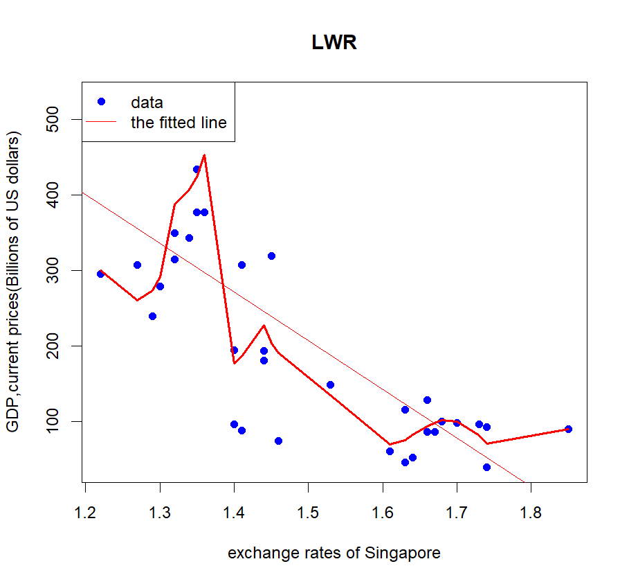
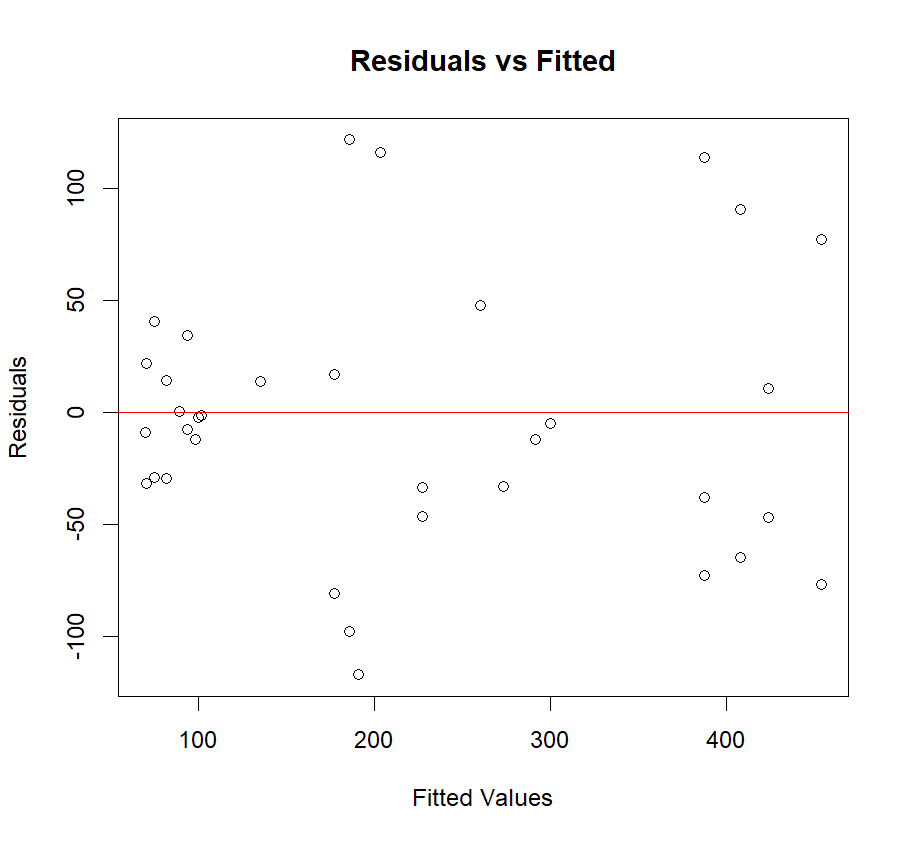
Figure 3: Left: the LWR and linear regression of exchange rates and GDP in Singapore; Right: the residuals versus the fitted values. The best span for Singapore is 0.3.

3.2. Results and Discussions

From these plots and residuals, the author discovered that the exchange rate and GDP of Japan has the strongest connection. Next is the Singapore. South Korea’s exchange rates have the weakest correlation with GDP [8]. These results are caused by various factors.

First and foremost, the economic structure. As known to all, Japan is an economy that relies heavily on exports, especially for manufacturing such as cars, electronics and machinery. Exchange rate changes directly affect its export competitiveness and thus have a significant impact on GDP. While Singapore is a city-state dominated by services and finance, with international trade and investment playing an important role in its economy. Singapore carries a managed floating exchange rate system, and exchange rate fluctuations are relatively controllable. Meanwhile, Although South Korea's economy is also dependent on exports (such as semiconductors, automobiles, and shipbuilding), its economy is relatively diversified and its domestic market is large, so it is less sensitive to exchange rate fluctuations.

Secondly, the policy also plays an important role. Japan has implemented loose monetary policies (such as quantitative easing) for a long time, resulting in large fluctuations in the yen exchange rate. Exchange rate fluctuations have a direct impact on GDP through trade channels. In contrast, The Monetary Authority of Singapore (MAS) manages the exchange rate in order to maintain price stability and economic growth, so the influence of the exchange rate on GDP is relatively indirect [9]. South Korea has a floating exchange rate, but the Bank of Korea steps into the global exchange market to secure the exchange rate and reduce the direct impact of currency fluctuations on the economy.

In addition, the influence of their trading partners cannot be neglected. Japan's vital trading partners (such as the United States and China) have a greater impact on its economy, and the impact of exchange rate changes on GDP through trade channels is more significant. Singapore and South Korea have relatively dispersed trading partners, and exchange rates have relatively little impact on GDP.

Moreover, the high relevance of Japan’s exchange rates and GDP has something to do with other factors, such as the opening degree in economics, industrial policies and historical background. Those factors conspire to bring about this result. In a nutshell, the dependency of GDP on exchange rates is determined by multiple elements, thus, it may give people a deeper insight into the difference of economic policies in Japan, South Korea and Singapore.

4. Conclusions

The author uses linear regression model and locally weighted regression method to analyze the association between exchange rates and GDP in Japan, South Korea and Singapore. Then the author finds that the exchange rate and GDP of Japan has the strongest connection. Next is the Singapore. South Korea’s exchange rates have the weakest correlation with GDP. Meanwhile, the author discusses the reasons of this results, which includes economic structures, policies and trading partners. Although the study discusses the relationship between exchange rates and GDP in those 3 countries, it has its own limitations. It only uses two models of regression and it does not compare the effect of different regression models. More regression models should be used in this study to find the best fit of the data. In the future, the author may focus on how exchange rates influence GDP. For instance, Future research could combine global value chain (GVC) statistics to figure out the impact of exchange rate movements on different parts of the global supply chain and how this effect is transmitted to GDP. Meanwhile, the pass-through impact of exchange rate fluctuation on prices and inflation is an important element affecting GDP. Future studies can further explore the asymmetry of exchange rate pass-through effects (such as whether the effects of exchange rate appreciation and depreciation are symmetrical) and its impact on GDP. Moreover, the author may further discuss the reasons for the difference of spans in these 3 countries.

References

[1]. Fan, Yen-Hui Fan, Wen-Ying Luo & Yuhang Zhang (2011). A new genus and species of the genus Pseudourostyla (Hymenoptera, Staphylinidae). (2025). Industrial structure and choice of exchange rate regime. Studies in International Finance, (02), 38-48.
[2]. Li Zhaochen, Han Tiankuo & Gao Yuning. (2024). International GDP Comparison and Relative Change Trend of Sino-US GDP. Journal of Guizhou University of Finance and Economics, (01), 11-20.
[3]. Liu, Xingtang & Liu, Jun. (2010). The dynamic relationship between real effective exchange rate, savings rate and GDP. Statistics and Decision Making, (01), 75-78.
[4]. Ross, S. M. (2019). A first course in probability (10th ed.). Pearson Education.
[5]. Sheather, S. J. (2009). A modern approach to regression with R. Springer.
[6]. Bishop, C. M. (2016). Pattern recognition and machine learning. Springer.
[7]. Husain, A. M., Mody, A., & Rogoff, K. S. (2005). Exchange rate volatility and economic growth: Evidence from developing countries. Journal of Economic Growth, 10(4), 1-21.
[8]. Bahmani-Oskooee, M., & Gelan, A. (2018). The impact of exchange rate movements on GDP growth: A comparative analysis of developed and developing economies. Journal of Economic Studies, 45(5), 1-20.
[9]. Levy-Yeyati, E., & Sturzenegger, F. (2023). Exchange rate regimes and economic growth: A panel data analysis. The World Bank Economic Review, 17(2), 1-24.
Cite this article
Huo,X. (2025). Impact of Exchange Rates of Japan, South Korea and Singapore on GDP. Theoretical and Natural Science,100,190-196.
Data availability
The datasets used and/or analyzed during the current study will be available from the authors upon reasonable request.
Disclaimer/Publisher's Note
The statements, opinions and data contained in all publications are solely those of the individual author(s) and contributor(s) and not of EWA Publishing and/or the editor(s). EWA Publishing and/or the editor(s) disclaim responsibility for any injury to people or property resulting from any ideas, methods, instructions or products referred to in the content.
About volume
Volume title: Proceedings of the 3rd International Conference on Mathematical Physics and Computational Simulation
© 2024 by the author(s). Licensee EWA Publishing, Oxford, UK. This article is an open access article distributed under the terms and
conditions of the Creative Commons Attribution (CC BY) license. Authors who
publish this series agree to the following terms:
1. Authors retain copyright and grant the series right of first publication with the work simultaneously licensed under a Creative Commons
Attribution License that allows others to share the work with an acknowledgment of the work's authorship and initial publication in this
series.
2. Authors are able to enter into separate, additional contractual arrangements for the non-exclusive distribution of the series's published
version of the work (e.g., post it to an institutional repository or publish it in a book), with an acknowledgment of its initial
publication in this series.
3. Authors are permitted and encouraged to post their work online (e.g., in institutional repositories or on their website) prior to and
during the submission process, as it can lead to productive exchanges, as well as earlier and greater citation of published work (See
Open access policy for details).