1. Introduction

1.1. Background

From ancient times to today, human cannot stop predicting what will the day be like for tomorrow. Methods include observing the cloud, putting salt in the camp fire, using pattern of empirical weather data, or training complex neural networks. These methods yield result forecasts that serve as important indicator with a wide range of downstream applications from choice of personal outfits, economic decisions, policy making, to natural disaster warning.

With the development of weather forecast techniques, weather forecast services with high precision and high resolution are available through the Internet. Users are able to receive features like temperature, precipitation, wind speed, thunder with complete GUI on mobile phones and personal computers. However, there are situations where internet might not be accessible or weather reports need to be forecasted locally. For example, volunteers preparing for possible flood during the internet outage following a severe earthquake, researchers in remote stations where the internet service provider is not always reliable, or a part of the offline failsafe serve an online weather forecasting service.

Such an offline method will require an acceptable processing time for quick forecasting and will limit input of data to a relatively short lookback window with only one source of data for isolated applications.

1.2. Current research

Chhetri et al. developed a BLSTM-GRU hybrid model that leverages bidirectional memory and gated recurrent units to improve monthly rainfall prediction in Bhutan, achieving lower mean square error than standalone deep learning models [1]. FuXi, proposed by Chen et al., is a cascaded machine learning system that extends skillful global weather forecasts up to 15 days, rivaling the ECMWF ensemble by reducing accumulated errors through multi-stage learning [2]. An attention-based sequence-to-sequence network from Setiawan et al. has been applied to indoor climate prediction, capturing temporal dependencies while improving accuracy through attention mechanisms [3].

Moreover, a transformer with shifted window cross-attention developed by Bojesomo et al. efficiently models spatiotemporal interactions in weather data, offering competitive nowcasting performance with fewer parameters [4]. The Bagging–XGBoost ensemble has been used for extreme weather identification and short-term load forecasting, enhancing grid stability by reducing error rates under peak load conditions [5]. LSTM networks have proven effective for short-term solar irradiance forecasting under complicated weather, outperforming traditional RNNs by mitigating gradient issues and better handling cloudy-day variability [6, 7].

1.3. Aim of the study

One might notice from the above research that they focus heavily on pre-trained complex models that requires numerous sensor inputs that could hinder usage like offline emergency or individual forecasting, which are limited by sole sensor input, slow computer and short lookback window.

To determine the performance of these weather forecasting methods in offline isolated situation, a comparative analysis is needed using a unified method with multiple metrics for a comparison across methods.

2. Methodology

2.1. Data preparation

For the training, validation, and evaluation, GSOD (Global Summary of the Day) from NOAA (National Oceanic and Atmospheric Administration) is selected since it provides daily weather information collected from ground weather stations. This data structure fits the target scenario of using an isolated sensor for forecasting. After removing flags, and station names, there are 7 relevant weather features and 4 space-time related stationary data selected. The sensor data include: temperature, precipitation, wind speed, dew point, station pressure, sea level pressure, and visibility. The stationary features are date, latitude, longitude, and elevation. The total cleaned dataset consists of 40 stations with data from 2000 to 2010.

For missing values, since total number of observations with not available value is less than 0.1 percent of the sample, all NA values are replaced using the mean value of the same station of the year. To avoid possible impact from the different unit of measure across feature, for example 10^1 for temperature but 10^3 for pressure, and later PCA (Principal Component Analysis) for dimensional reduction, all features are normalized compare to the range of the total sample space.

2.2. Training

The scaled input for every model is consisted of 90 days of 7 weather features and 4 static features. The output is horizon with 15 days of 4 weather features include temperature, precipitation, visibility, and wind speed. The training/evaluation set is divided to 9:1. All deep learning models are trained with the following common hyperparameters as shown in Table 1.

To train all deep learning model, a Python 3.12 module in is called. The module prepared the dataset and used the above hyperparameters to call different methods of trainers. Also, to prevent overfitting, method of early stopping is used with patience 8 with validation set. In event of validation MSE not improving for 8 epochs, the training process stops and yield the model with lowest validation MSE. For evaluation, a similar module as the training module is called and evaluate the models saved after training. The evaluation module uses sliding windows with the same IO as in training and calculate the result metric for performance comparison. The specific setup for each Deep Learning methods is outlined in provided code.

The test on the performance of traditional Machine learning methods involves three renowned methods. Persistence Model, where the forecast result is the same as the day before, is used as a baseline model here. Linear Regression is included for its simplicity and its ability to capture linear relation. The other one is XGBoost, a tree-based method that is excellent is accuracy and fast in speed. All of the traditional methods used PCA for dimensional reduction with more than 90% of explained variance given the fact that 90*7+4 inputs is very computational heavy for methods like XGBoost. Moreover, all traditional methods are trained for each of 4 result features independently for three horizons: Day 1, 7 and 15.

2.3. Metrics

The performance metric is consisted of Nash–Sutcliffe, an R^2-like skill that measures how well model predictions match observed data, relative to the mean of the observations

$$ Skill = 1-\frac{\text{MSE}}{\text{Var}\left(y_{true}\right)}$$(1)

Root Mean Square Error (RMSE) is also used to quantify the average magnitude of errors between observed and predicted values [8]. It is useful when large errors are particularly undesirable, giving higher weight to larger deviations.

$$ \text{RMSE}=\sqrt{\frac{1}{n}{\sum }_{i=1}^n{\left(y_{true}-y_{est}\right)}^2}$$(2)

Evaluating with NSE and RMSE is complementary: NSE measures errors against climatology (the station mean), while RMSE for to absolute magnitude. For low-variance settings, NSE is sensitive to small error changes; for skewed targets like precipitation, RMSE can be dominated by rare larger events. Reporting both, per variable and horizon, was therefore suitable.

Since the application scenario demands limitation on computational power, the total time of making forecasting is also measured to compare the cost of inferencing using pre-trained models.

3. Results

3.1. Overview

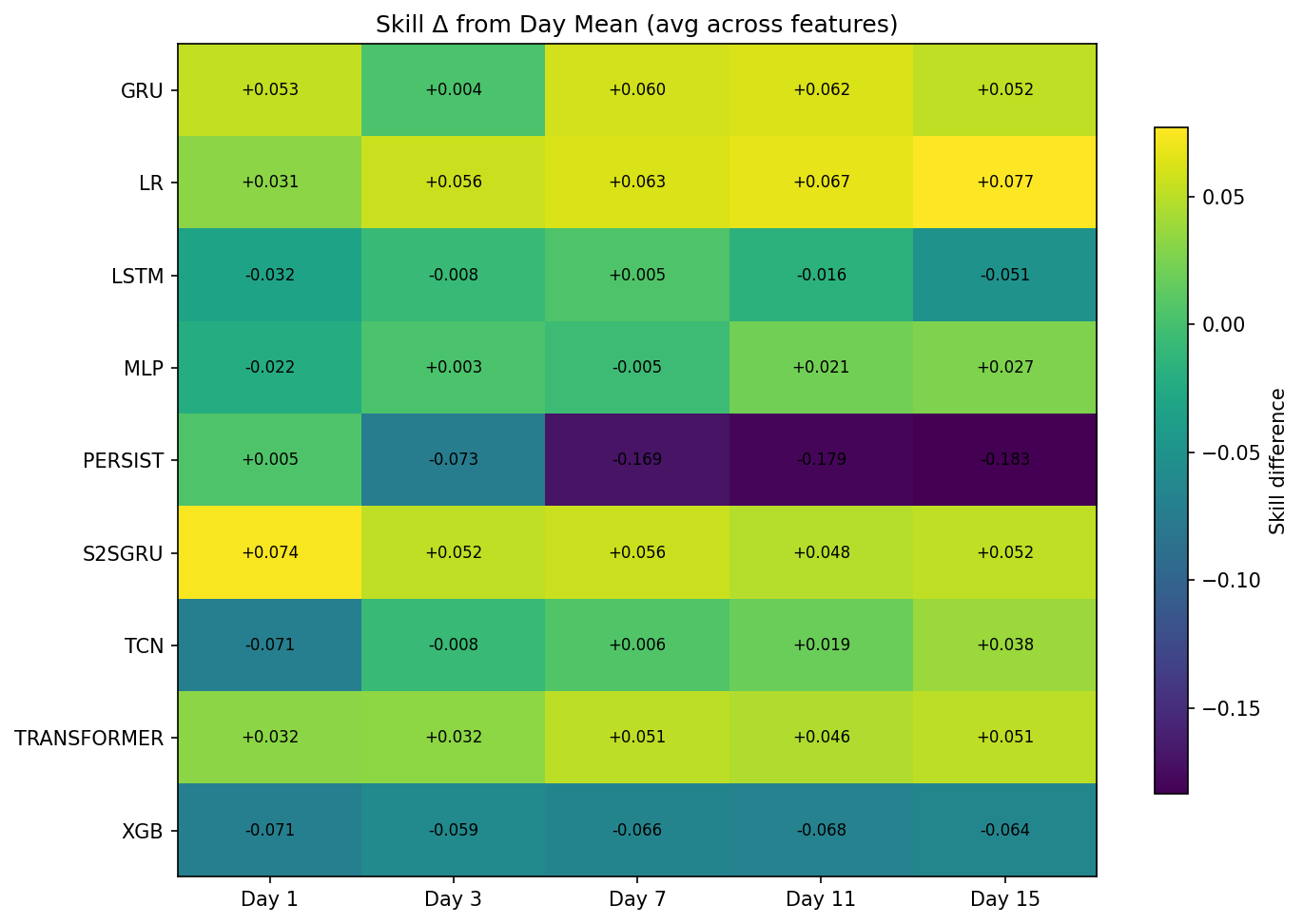
As shown in Figure 1, the above is the heatmap showing the comparative overall skill of models. It shows the naïve Persistence performs the worse overall with expected failure as the horizon increases. The XGBoost also performed poorly compare to the daily average. Models with significant positive skill compare to the average are LR, S2SGRU, and Transformer. The statistics in each block is calculated by comparing the mean of average skill of all features for each model each day and the average skill of features for any model.

3.2. Performance per feature

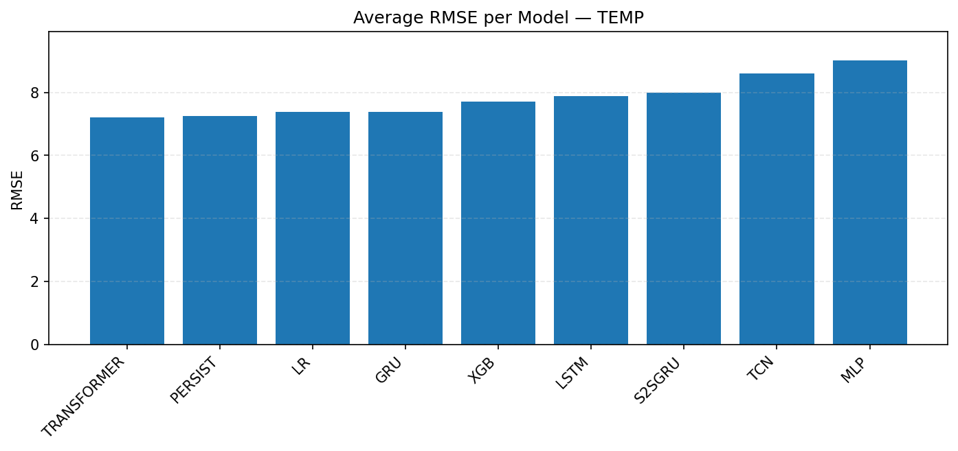
For temperature (TEMP), as shown in Figure 2, the best model is Transformer with RMSE around 7.2. Persistence, LR, and GRU are just behind in the same narrow range. XGB and LSTM are modestly worse at about 7.4–7.6. S2SGRU is a bit weaker here at 7.7, and both TCN and MLP underperform, with MLP the worst at about 9.0.

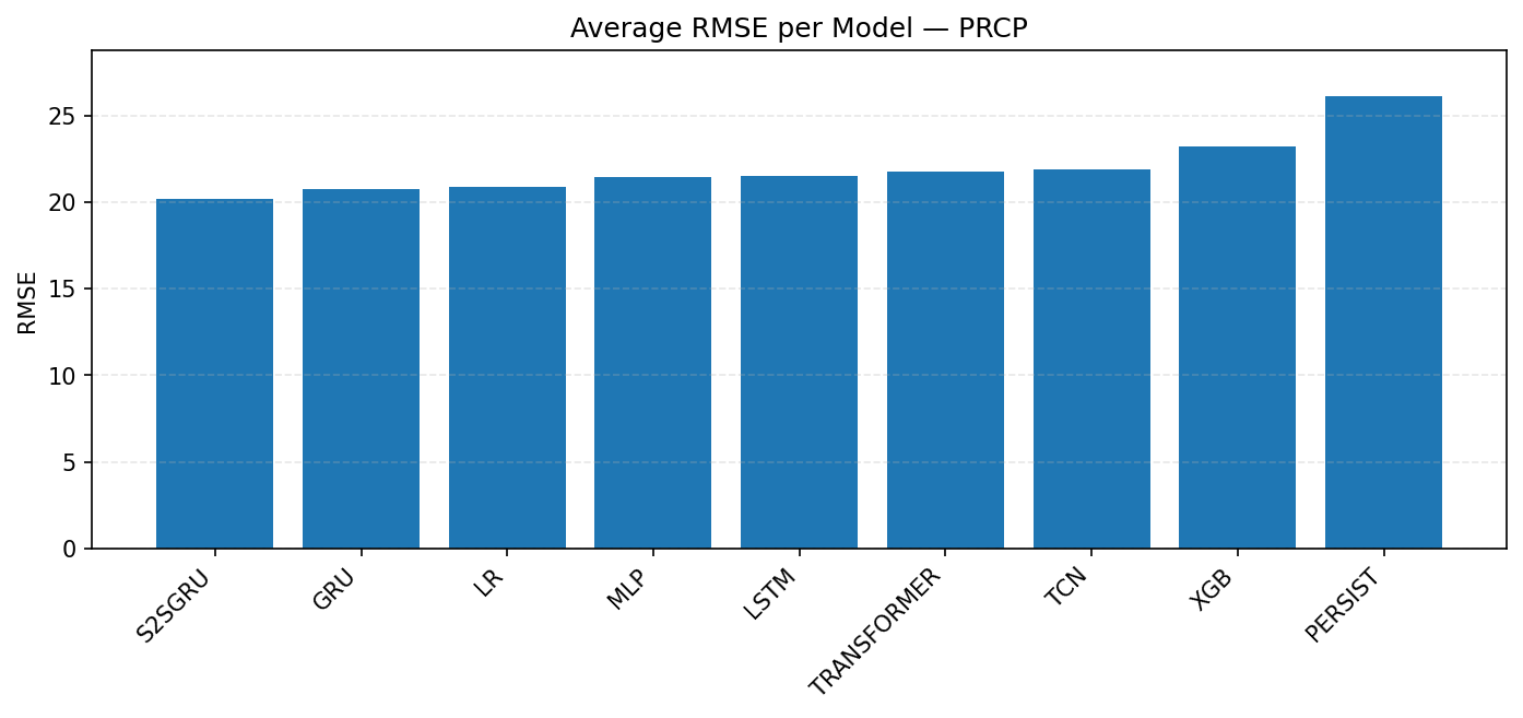
From Figure 3, the best performance for precipitation is from S2SGRU, with RMSE near 20, and GRU closing behind. A middle cluster of models consist of LR, MLP, and LSTM is within the 21–22 range, with Transformer and TCN similar but slightly weaker. The poorest models here are XGB, which increased toward 23, and Persistence, which collapses entirely at about 26. This fits with the earlier conclusion that S2SGRU excels on precipitation while Persistence is not viable.

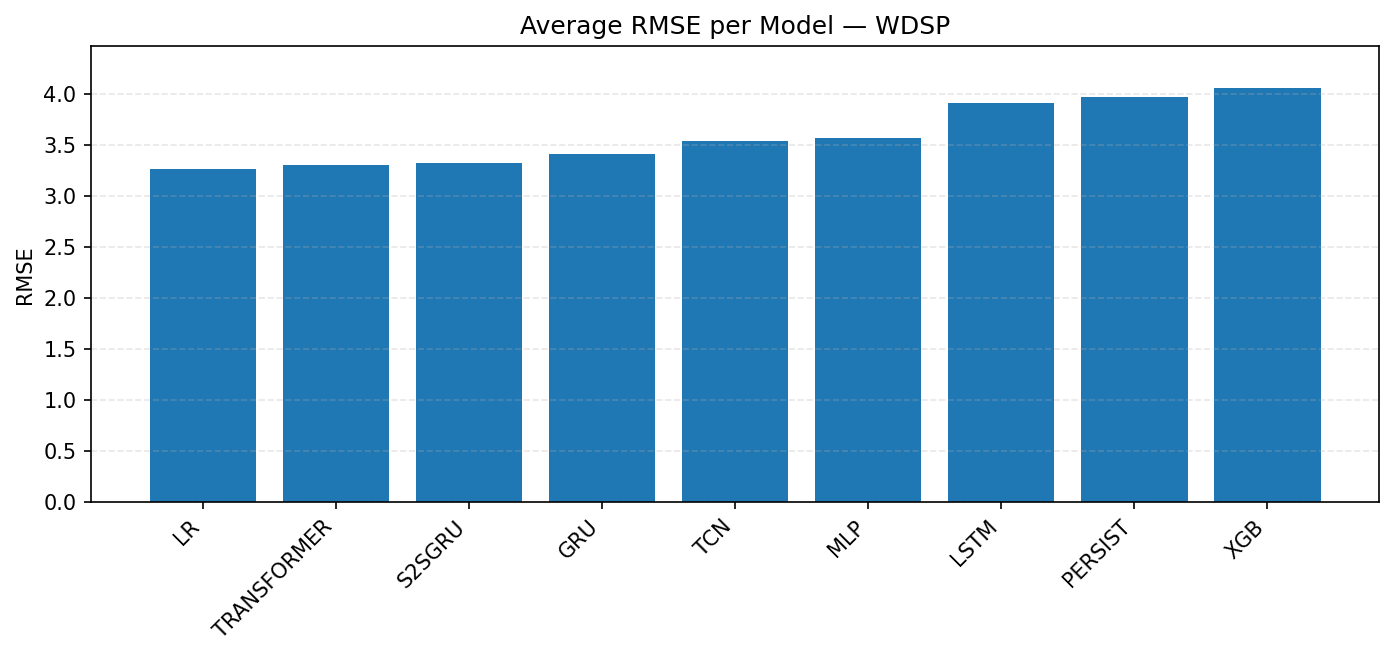
For wind speed (WDSP), the lowest RMSE in Figure 4 comes from LR, followed very closely by Transformer, S2SGRU, and GRU. All of them stay around the 3.2–3.3 range. A second tier includes TCN, MLP, and, which are slightly higher around 3.5–3.6. The weakest models are LSTM, Persistence and XGBoost, which rise to 3.9 and above 4.1 respectively. Thus, LR is the most reliable choice for WDSP, and XGBoost perform poorly.

As in Figure 5, the lowest overall RMSE of visibility is achieved by S2SGRU, GRU, and LR, all clustered around 4.9–5.0. Transformer follows closely at about 5.0, then LSTM and MLP a bit higher near 5.2–5.3. TCN and XGB are worse with around 5.8. Persistence is again the worst, above 6.3. This shows S2SGRU is comparatively effective for visibility, with LR and GRU nearly tied.

3.3. Performance per day

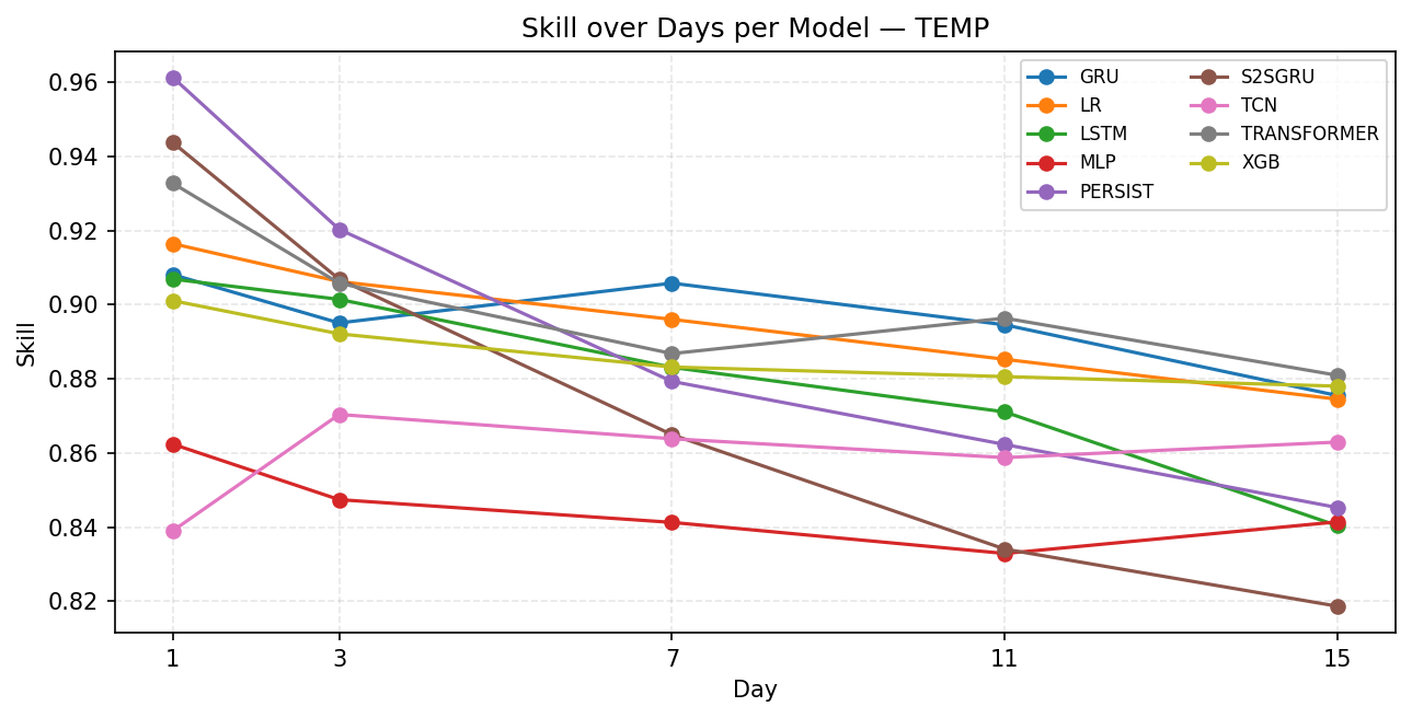
As for skill, Figure 6 shows that in temperature, all models lose skill as the forecast horizon increases, which is expected in time series forecasting. Persistence model starts the highest (around 0.96), because at short horizons the naïve assumption works very well. S2SGRU, Transformer, LR also begin very strong (>0.92). In stability, GRU, LR, Transformer, and XGB decline gradually, which suggest they are more reliable over longer horizons. S2SGRU and PERSIST drop sharply, suggesting strong in very short-term, poor in medium/long-term. Also note that LSTM declines steadily but performs worse than GRU, and MLP hovers at the bottom throughout (~0.84–0.86), showing weak performance overall.

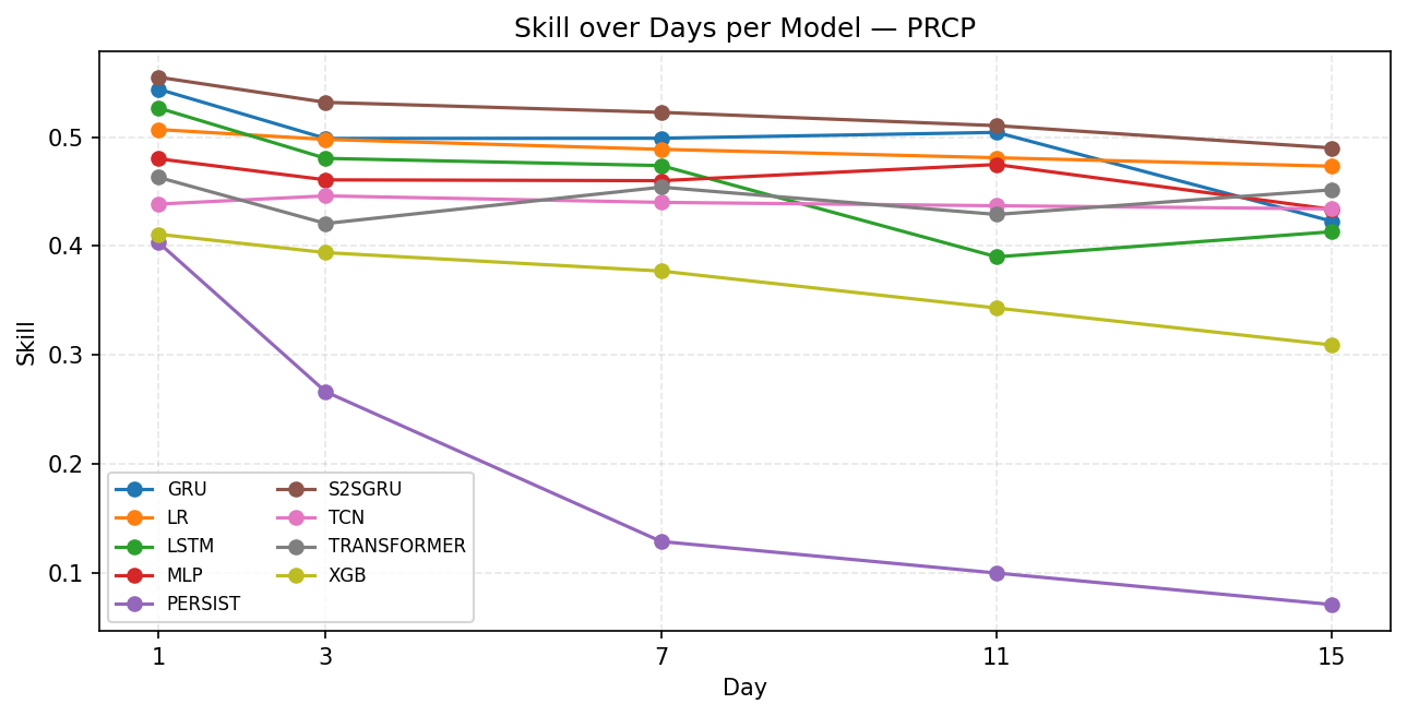
Clearly forecasting PRCP is harder than TEMP with the skills on the graph is now ranged from 0.3 to 0.55, compare to above 0.82 for TEMP, as demonstrated in Figure 7. Most of the models perform consistently throughout the horizon from skill 0.4 to 0.55 with S2SGRU being the best among the models. The XGBoost still perform the badly but not as terrible as the Persistence model that holds skill less than 0.1 in day 15.

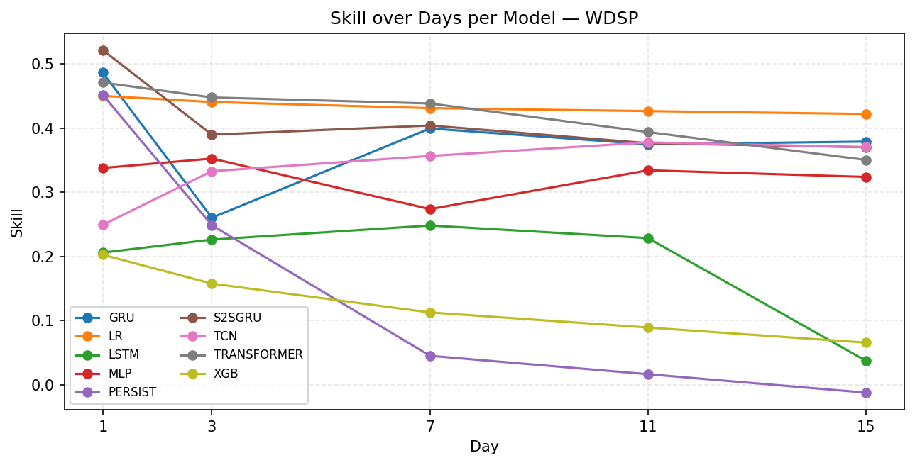
As for wind speed, LR in Figure 8 is the clearly with best performance and the most stable across horizons. For start to mid-horizon, Transformer is also strong around 0.45, close to LR. S2SGRU, GRU start very high around 0.5 but collapse by Day 3–15 to around 0.35. Note that performance of MLP gradually improve over horizon. LSTM struggles, peaking at around 0.25 then collapsing on Day 15 to around 0.03. PERSIST and XGB is not performing well and Persistence even shows sign of negative skill at day 15.

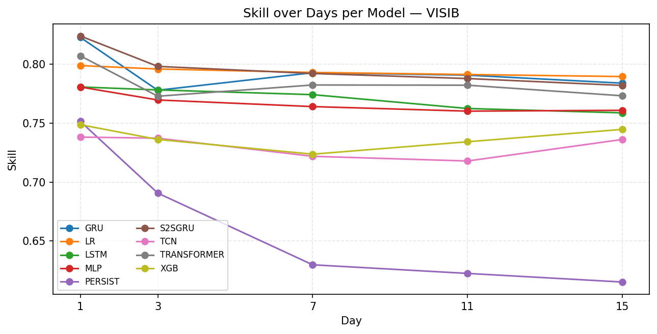
For visibility, S2SGRU, GRU, LR, TRANSFORMER in Figure 9 all stay strong around 0.78 to 0.80 across horizons. LR is noticeably the most stable one that barely declines. LSTM, MLP settle around 0.76, slightly below the top models. TCN and XGBoost stays around 0.74 lower than other models. Persistence collapses badly from 0.75 to around 0.64.

3.4. Performance in speed

Table 2 shows the measurement of the inference process, which is taken with average of three trial. The time does not contain the preprocessing of data.

As shown in the table, the LR (Linear Regression) shows the least inference time. MLP and GRU maintained about 500 to 600 milliseconds, while most of other methods exceed 1000 milliseconds.

Therefore, looking across all variables, LR is remarkably consistent. It has top or near-top results in every case, and stands out especially for wind speed. S2SGRU is a standout for precipitation and visibility, but less competitive for temperature. GRU is a strong all-rounder, competitive across PRCP, VISIB, and WDSP, though slightly behind Transformer for TEMP. Transformer itself is the best for temperature and very solid for wind speed, but more mid-range for precipitation and visibility. MLP and TCN are generally mediocre. XGB consistently struggles and shows higher RMSE values across the board. Lastly, Persistence only works acceptably for very short-term temperature but fails on other variables and especially poor with horizon larger than 1.

4. Discussion

The study has compared traditional and deep learning approaches for 15-day, multi-target forecasting from single-station daily observations (GSOD). Several consistent patterns emerge across variables and horizons.

Firstly, Transformer and S2S/GRU architectures, which features in model temporal dependencies, yield clear gains over naïve and tree-based baselines. Transformer is strongest for temperature, a highly autocorrelated (as shown in day 1 persistence), smooth signal for which long-range attention is advantageous. S2SGRU excelled on precipitation and visibility, variables that benefit from regime/context modeling and short-to-medium memory. However, gains were not universal: for wind speed, a simple linear regression (LR) matched or slightly outperformed the deep models, suggesting that WDSP dynamics in these data are close to linear given the chosen inputs and 90-day context window.

Secondly, LR is a surprisingly strong and stable performer across variables and horizons, often top-2 and the best on wind speed. In contrast, XGBoost consistently lack such performance. Although PCA is friendly to LR by compressing the inputs while keeping over 90 percent of variance, and significantly cut the training time of the trees, it could degrade tree models by mixing features, especially for the temporal structure, into dense linear components that are less separable via splits due to the structure of trees.

Thirdly, all models lose skill with increasing horizon. This is an expected outcome for multi-step forecasts, but the slope of degradation varies. Transformer and LR decline gradually for temperature, indicating more reliable longer-range behavior. S2SGRU shows sharper drops on some targets like precipitation beyond a few days, consistent with sequence-to-sequence models that capture short-term context very well but may overfit to short-horizon dynamics or suffer from exposure to distributional shift across the 15-step outputs.

5. Conclusion

Using 90 days of station-local GSOD inputs to forecast 15 days across four targets features, the results are:

1. Linear Regression is a strong, low-latency baseline, winning wind speed and tying near the top for visibility, while remaining competitive for temperature and precipitation.

2. Transformer achieves the best temperature skill and maintains accuracy with horizon, consistent with its strength in long-range dependencies.

3. S2SGRU is best for precipitation and visibility, leveraging sequence modeling to capture short-to-mid-range regimes, though its skill declines steeply at longer horizons on temperature.

4. XGBoost underperforms in this setup, likely due to PCA compression (thought PCA only saves above 90% of explained variance) and lack of temporal inductive bias—and persistence is only viable for Day-1 temperature.

For an application constrained by compute, a variable-aware portfolio is recommended: LR for wind speed (and often visibility), Transformer or GRU for temperature as budget allows, and S2SGRU for precipitation.

Future work could focus on uncertainty quantification, combination of models, exogenous predictors, and other station-robust evaluation. These steps are likely to yield additional, deployment ready improvements without abandoning the isolated-sensor constraint.

References

[1]. Chhetri, M., Kumar, S., Roy, P. P., & Kim, B.-G. (2020). Deep BLSTM-GRU model for monthly rainfall prediction: A case study of Simtokha, Bhutan. Remote Sensing, 12(19), 3174.
[2]. Chen, L., Zhong, X., Zhang, F., Cheng, Y., Xu, Y., Qi, Y., & Li, H. (2023). FuXi: A cascade machine learning forecasting system for 15-day global weather forecast. npj Climate and Atmospheric Science, 6, 190.
[3]. Eka Setiawan, K., Elwirehardja, G. N., & Pardamean, B. (2023). Indoor Climate Prediction Using Attention-Based Sequence-to-Sequence Neural Network. Civil Engineering Journal, 9(5), 1105–1120.
[4]. Bojesomo, A., Al Marzouqi, H., & Liatsis, P. (2024). A novel transformer network with shifted window cross-attention for spatiotemporal weather forecasting. IEEE Journal of Selected Topics in Applied Earth Observations and Remote Sensing, 17, 45–55.
[5]. Deng, X., Ye, A., Zhong, J., Xu, D., Yang, W., Song, Z., Zhang, Z., Guo, J., Wang, T., Tian, Y., Pan, H., Zhang, Z., Wang, H., Wu, C., Shao, J., & Chen, X. (2022). Bagging–XGBoost algorithm-based extreme weather identification and short-term load forecasting model. Energy Reports, 8, 8661–8674.
[6]. Yu, Y., Cao, J., & Zhu, J. (2019). An LSTM short-term solar irradiance forecasting under complicated weather conditions. IEEE Access, 7, 145651–145666.
[7]. Sherstinsky, A. (2020). Fundamentals of recurrent neural network (RNN) and long short-term memory (LSTM) network. Physica D: Nonlinear Phenomena, 404, 132306.
[8]. Chicco, D., Warrens, M. J., & Jurman, G. (2021). The coefficient of determination R-squared is more informative than SMAPE, MAE, MAPE, MSE and RMSE in regression analysis evaluation. Peerj computer science, 7, e623.
Cite this article
Lai,H. (2025). Comparing Machine Learning Methods for Offline Applications with Short Lookback and Limited Input. Theoretical and Natural Science,132,33-42.
Data availability
The datasets used and/or analyzed during the current study will be available from the authors upon reasonable request.
Disclaimer/Publisher's Note
The statements, opinions and data contained in all publications are solely those of the individual author(s) and contributor(s) and not of EWA Publishing and/or the editor(s). EWA Publishing and/or the editor(s) disclaim responsibility for any injury to people or property resulting from any ideas, methods, instructions or products referred to in the content.
About volume
Volume title: Proceedings of CONF-APMM 2025 Symposium: Simulation and Theory of Differential-Integral Equation in Applied Physics
© 2024 by the author(s). Licensee EWA Publishing, Oxford, UK. This article is an open access article distributed under the terms and
conditions of the Creative Commons Attribution (CC BY) license. Authors who
publish this series agree to the following terms:
1. Authors retain copyright and grant the series right of first publication with the work simultaneously licensed under a Creative Commons
Attribution License that allows others to share the work with an acknowledgment of the work's authorship and initial publication in this
series.
2. Authors are able to enter into separate, additional contractual arrangements for the non-exclusive distribution of the series's published
version of the work (e.g., post it to an institutional repository or publish it in a book), with an acknowledgment of its initial
publication in this series.
3. Authors are permitted and encouraged to post their work online (e.g., in institutional repositories or on their website) prior to and
during the submission process, as it can lead to productive exchanges, as well as earlier and greater citation of published work (See
Open access policy for details).