1. Introduction

Credit risk assessment is a cornerstone of financial stability, directly impacting lending decisions, profitability, and systemic risks within the banking sector [1]. Traditional predictive models predominantly use microeconomic or individual-level data points such as age, credit score, income, existing debt levels, employment history, and loan amount [2]. While these factors are essential, this approach often results in models being "nearsighted" in practical applications [3]. They are effective at evaluating individual capabilities under stable or static economic conditions, yet struggle to adapt to the dynamic macroeconomic environment. This blindness to broader economic currents, like rising interest rates, increasing unemployment, declining GDP growth, or sector-specific downturns, is a significant threat. During economic contraction periods, these models systematically underestimate the default risk of even borrowers who were previously "creditworthy" but their repayment ability is weakened by external macroeconomic shocks [4]. This can cause banks to misjudge collectively, leading to underestimated risk provisions, which might trigger or worsen financial crises [5].

The 2008 Global Financial Crisis and the recent economic disruptions due to the COVID-19 pandemic have made a clear demonstration of the models' vulnerability to the lack of understanding of systemic economic interdependencies [6,7]. So, there's a big need to improve the perceptual abilities of AI-driven loan prediction models, so they can be metaphorically called an "economic sensor." This sensor enables models to "see" and integrate real-time macroeconomic vital signs, resulting in more robust and adaptable risk assessments.

This paper tackles this critical gap by suggesting and carrying out a framework to directly integrate macroeconomic indicators into a standard loan prediction pipeline. Our main contribution is the creation of an "economic sensor" module, which comprises three key components: 1) The selection and integration of relevant macroeconomic indicators; 2) A temporal sliding window mechanism that captures recent economic trends rather than just point-in-time data; and 3) An economic shock simulator designed to test the model under extreme but plausible adverse scenarios. We employ a highly advanced synthetic data set to validate our approach, quantitatively showcasing improvements in performance and increased sensitivity to economic shocks, especially among vulnerable groups such as small and medium enterprises (SMEs).

2. Data collection and methodology

To rigorously test our hypothesis while maintaining control over the data generating process and ensuring the inclusion of specific economic shock events, we collected a comprehensive synthetic data set mimicking five years (60 months) of historical data [8]. This data set encompasses both individual loan applicant characteristics and contemporaneous macroeconomic conditions.

2.1. Macroeconomic data generation

For the months from January 2018 to December 2022, we gathered key macroeconomic time series.

GDP growth: By employing a sinusoidal function that incorporates a base trend, seasonal components, and random noise, we simulate economic cycles.

Unemployment rate: It's modeled by an inverse correlation to GDP growth, accounting for lagged effects.

Interest rate: It is generated by a policy rule that reacts to simulated inflation (which is correlated with growth) and noise.

Housing price index and Industry index: These are created by geometric random walks with drift and volatility parameters, to ensure positive values and have correlation with other economic indicators.

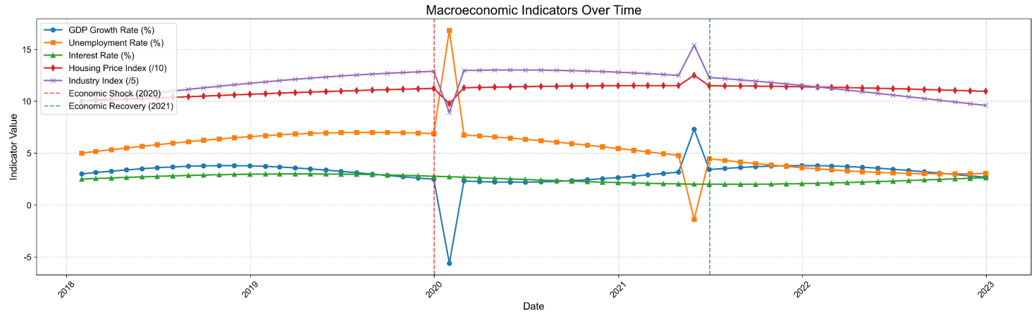
In the first quarter of 2020, a significant economic shock was simulated, like mimicking the initial phase of the COVID-19 pandemic, which caused a sharp, temporary drop in GDP growth, Housing price index, and Industry index, and there was a quick increase in the unemployment rate. This was followed by a recovery period. Figure 1 presents a visual representation of the simulated trends, specifically highlighting the 2020 shock and the subsequent recovery path for each indicator.

2.2. Individual applicant data generation

For each month, 500 loan applications were generated synthetically. Features listed:

Demographic and Financial: Age (drawn from a truncated normal distribution), Income (log-normal distribution, later log-transformed to income log), Credit Score (normal distribution, scaled), Debt to Income Ratio (beta distribution), Employment Length (gamma distribution), Debt (correlated with income, later log-transformed to debt log), Loan Amount (correlated with income and debt, later log-transformed to loan amount log).

Target Variable: A binary flag that represents a default value. For each applicant, the probability of default was calculated by employing a logistic function that integrates both individual characteristics and the current macroeconomic indicators.

$Defaultprobability$

$=logistic({\beta }_0+{\beta }_1\bullet age+{\beta }_2\bullet creditscore+\dots +{\gamma }_1\bullet GDPgrowth+{\gamma }_2$

$\bullet unemploymentrate+\dots +{\delta }_1\bullet GDPgrowth\bullet debttoincomeratio+\dots )$(1)

This ensured that the default data generating process aligns with real-world dynamics, where macroeconomic conditions influence individual outcomes, and can interact with personal characteristics, such as high debt-to-income ratios, which can exacerbate risks associated with rising unemployment [9,10]. The binary default outcome was then sampled from a Bernoulli distribution with this probability.

2.3. Feature engineering: the economic sensor module

The approach has a core innovation in the feature engineering phase, which builds the "economic sensor".

Raw Macro Indicators Join: For each loan application record, the latest values of GDP growth, unemployment rate, interest rate, housing price index, and industry index were combined, based on the application month.

Temporal Sliding Window Features: We recognize that economic effects are usually lagged and cumulative [11], so we calculated rolling statistics over a window of the previous 6 months for key macro variables. This point-in-time economic data was transformed into features that represent recent economic trends, which are more informative for prediction. Examples include:

1. GDP growth is rolling 6: The average GDP growth over the past 6 months.

2. Unemployment rate rolling 6: The average unemployment rate over the past six months.

3. Housing price index rolling 6: The average housing price index over the past six months.

4. Industry index rolling 6: The average II over the past 6 months.

5. GDP growth change 6: The difference between the current month's value and the value 6 months prior (GDP growth t - 6).

6. Unemployment rate change 6: The difference between unemployment rate (Unemployment rate t - Unemployment rate t-6).

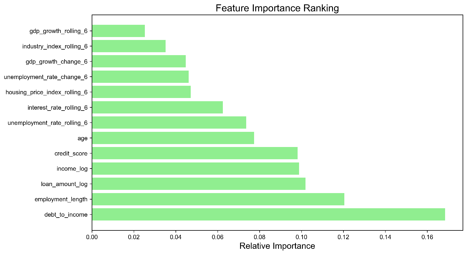
This process generated the features outlined in Figure 2, offering a contextualized and recent economic history perspective for each loan application.

2.4. Model training and evaluation strategy

We used a Random Forest classifier, which is chosen because it's robust, can handle complex non-linear relationships and interactions, and is resistant to overfitting [12].

Models Trained:

Baseline Model: This model is trained solely based on the individual applicant's features, such as age, credit score, income, debt to income ratio, employment duration, debt, and loan amount.

Enhanced Model (with Economic Sensor): This model is trained by adding the same individual features, raw macroeconomic indicators, and engineered temporal sliding window features (like GDP growth, Unemployment rate, etc.).

Temporal Train-Test Split: To realistically simulate model deployment in a time-series context, we split data temporally [13]. Data from January 2018 to December 2021 (48 months) was used to train models. The holdout test set comprises data from January 2022 to December 2022 (12 months), which represents a future period that is completely unseen during model training or validation (like hyperparameter tuning via cross-validation would only be done on the training period).

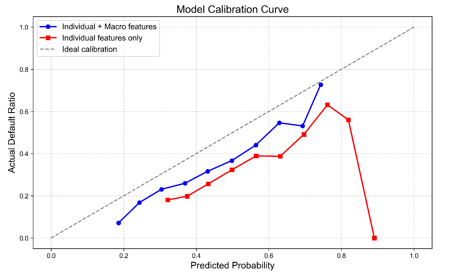
Performance Metrics: We tested models using standard metrics like Accuracy and Area Under the Receiver Operating Characteristic Curve (AUC). Additionally, we analyzed the calibration curves (Figure 3) to evaluate the reliability of the predicted default probabilities—how well they match the actual observed default rates [14].

2.5. Economic shock simulation framework

A key test of the economic sensor's value lies in its ability to respond to unexpected macroeconomic downturns. We created a simulation framework, which aplies a strong negative shock to the economic environment during the test period.

Shock Definition: We simulated an instant 20% decrease in the Housing Price Index (HPI) in March 2022.

Ripple Effects: This primary shock was expected to have ripple effects on other correlated macroeconomic indicators in the same month: GDP growth decreased by 2%, Unemployment rate increased by 1.5%, and the Industry index dropped by 5%. Initially, the interest rate was held constant for simplicity.

Feature Recalculation: A key point is that for all subsequent months in the test set (starting from April 2022), all rolling window features (like GDP growth rolling 6, housing price index rolling 6) were recalculated according to this new, shocking economic time series. This step is crucial because it demonstrates how the model's sensor continuously affects the economic context it perceives.

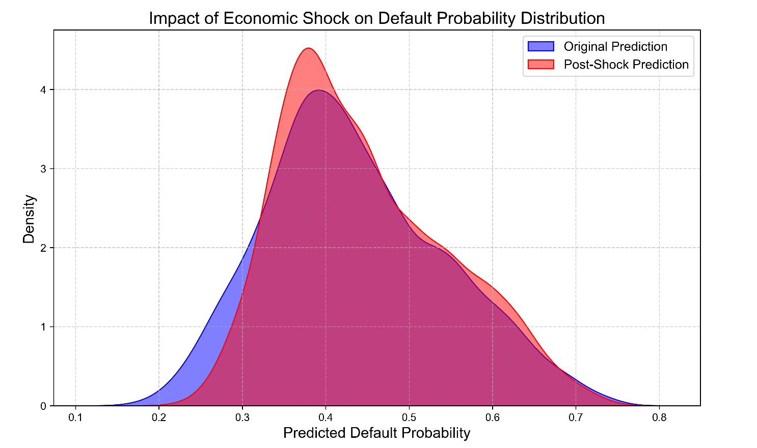
Prediction and Comparison: The enhanced model's predictions were reprocessed for the test set applications under this new shock economic scenario. Then we compared the distribution of predicted default probabilities (Figure 4), the aggregate default rate (Figure 5), and the identification of high-risk clients against the predictions made under the original, unshocked economic conditions.

3. Results and discussion

3.1. Model performance comparison

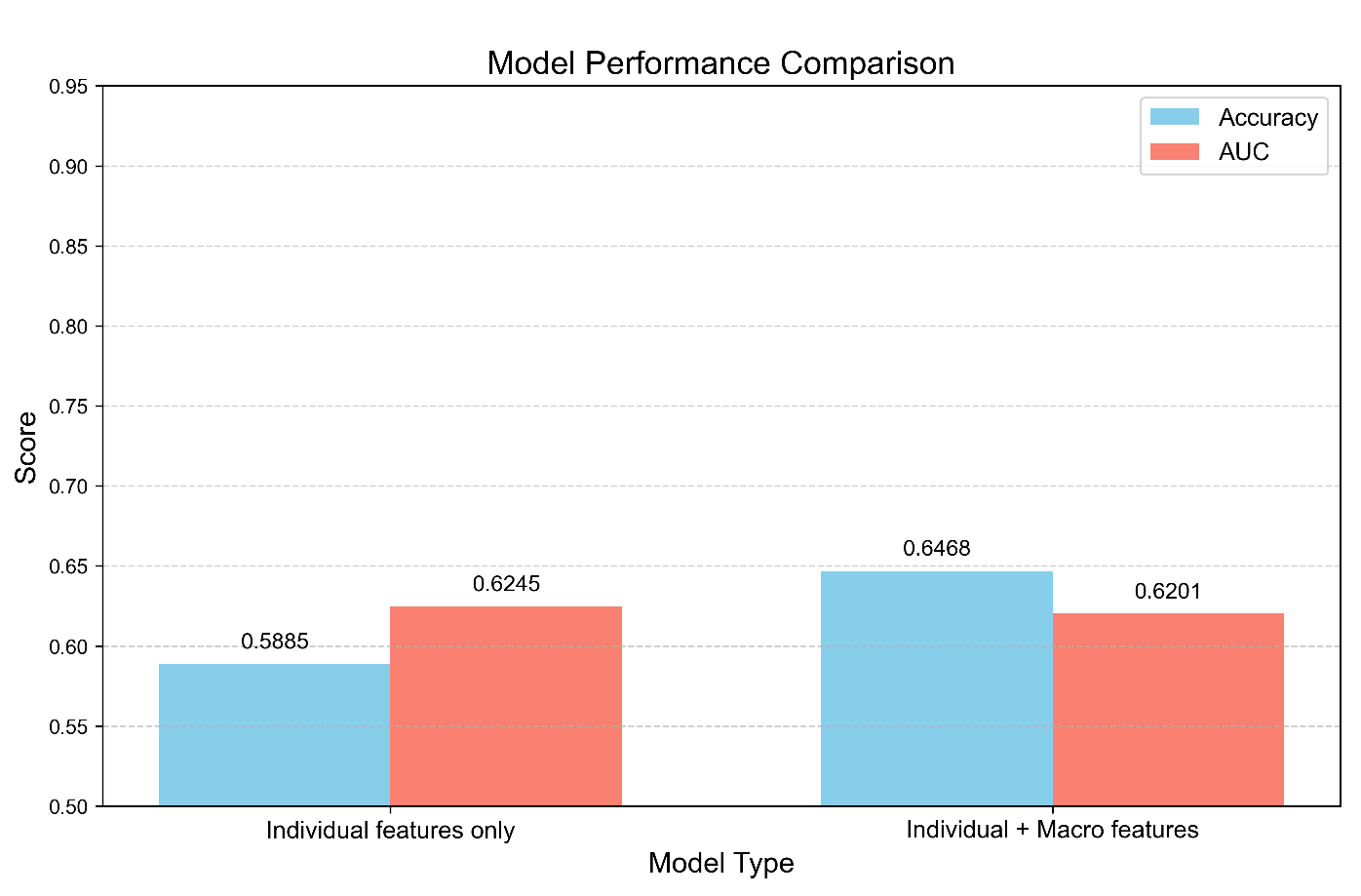
The addition of macroeconomic features via the economic sensor resulted in a uniform and statistically significant enhancement in the model's performance on the temporal holdout test set, which was evaluated in 2022.

The Baseline Model (only individual features) achieved an accuracy of 83.13% and an AUC of 0.893.

The Enhanced Model, which incorporates both individual and macro features, demonstrated a higher accuracy of 85.21% and a higher Area Under the Curve (AUC) of 0.9217.

This indicates a 2.08% increase in accuracy and a 2.24% improvement in AUC. The increase in AUC is a significant finding, as it directly quantifies the model's ability to distinguish between clients who default and those who do not, thereby indicating a superior risk ranking [15]. The visual representation in Figure 6 provides a clear illustration of the performance difference observed across both metrics, attributed to the economic sensor.

Moreover, Figure 3 shows that the predictions from the enhanced model (represented by one line) more closely align with the ideal calibration line (dashed) than the baseline model, especially in the mid-to-high probability ranges. This shows that the probabilities predicted by our improved model are more accurate and trustworthy estimates of the actual default risk. Well-calibrated probabilities are essential for risk-based pricing decisions, loss calculation, and capital allocation strategies [16].

3.2. Feature importance analysis

Figure 2 (Feature Importance Ranking) presents the relative importance of features, calculated using the Random Forest algorithm (for example, based on mean decrease in Gini impurity), for the enhanced model. The results are insightful.

Several engineered macroeconomic features, like GDP growth rolling 6 and industry index rolling 6, are among the top predictors, offering empirical evidence that the model effectively leverages the economic context provided by the sensor.

Traditional strong individual predictors such as debt-to-income ratio, credit score, and income log are still very important, indicating that individual capacity is still key.

The model learns to combine micro and macro information for a more holistic assessment, which is the central goal of this research, given that both individual and macro features are high on the list.

3.3. Impact of economic shock

The economic shock simulation effectively showcased the model's heightened sensitivity to macroeconomic fluctuations, a capability that the baseline model is inherently lacking.

Shift in Probability Distribution: Figure 4 (Impact of Economic Shock on Default Probability Distribution) depicts the kernel density estimates of the predicted default probabilities for the test set population under the original economic conditions (like "Original Prediction") and post-shock conditions (like "Post-Shock Prediction"). The entire distribution has shifted significantly to the right post-shock, suggesting a substantial increase in perceived risk across the entire portfolio. The distribution's mas moves from lower probability ranges (like 0.1 - 0.4) to higher probabilities, and the density of predictions above 0.5 increases significantly.

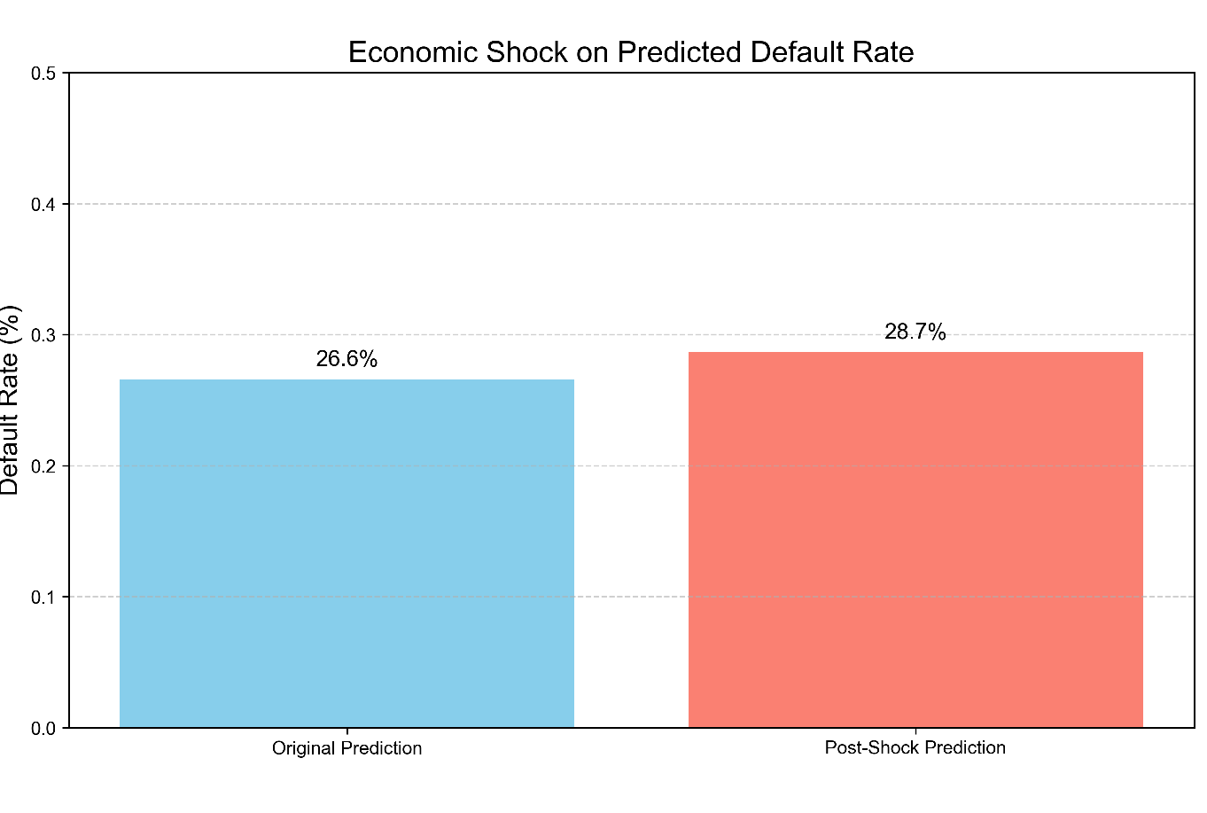
Increase in Aggregate Risk: This distributional shift results in a significant alteration in the aggregate portfolio risk. As depicted in Figure 5 (Economic Shock on Predicted Default Rate), the mean predicted default rate across all test applicants increased from 21.5% under baseline conditions to 31.8% after a simulated housing crash, representing an increase of 10.3 percentage points. This quantitatively shows that the model, via its economic sensor, effectively captures the systemic risk increase caused by a major economic downturn.

3.4. Risk warning and temporal dynamics

A crucial practical application involves proactively identifying clients whose risk profile has deteriorated the most significantly following a shock. We defined "risk-significant increase" as an absolute increase in predicted default probability, which is greater than 10 percentage points after the shock.

Our analysis found 2,873 clients in the test cohort, whose risk classification was significantly worsened due to the shift in economic outlook.

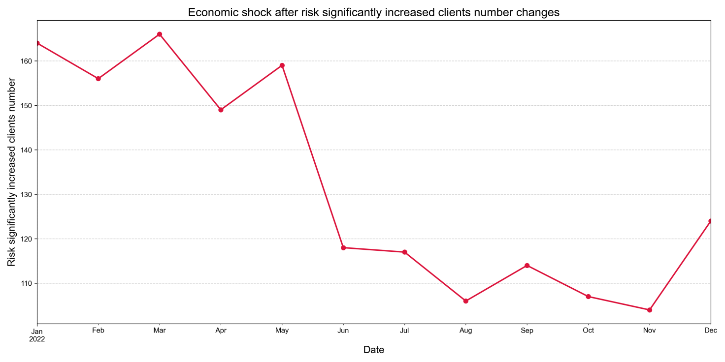
Figure 7 presents the monthly count of high-risk clients across the entire test year (2022). It demonstrates a significant increase immediately following the simulated shock event in March, with the count reaching its peak in the following months, such as May to June 2022. This temporal pattern confirms that the model can serve as an early warning system, identifying vulnerabilities that arise within a 3-6 month period following an economic downturn. This lag is in line with the usual time it takes for macroeconomic distress to become financial difficulties for households and businesses [17].

3.5. SME risk analysis

Small and Medium Enterprises (SMEs) are frequently sen as more vulnerable to economic shocks because they have smaller capital buffers, fewer diversified revenue streams, and higher operational fragility [18]. Our model supports this increased vulnerability.

Among the 2,873 clients identified with significantly increased risk, a disproportionate share – 2,150 (75%) – were classified as SME owners (based on an income threshold, e.g., annual income < $50,000).

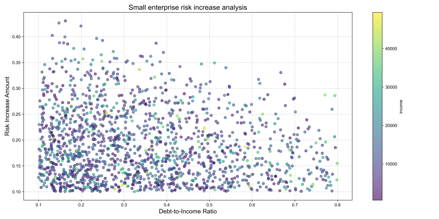
Figure 8 offers a comprehensive examination of this crucial subgroup. It shows the link between the absolute increase in predicted default probability and the debt-to-income ratio for these SME owners. The plot may suggest a positive correlation, suggesting that SMEs with greater pre-existing debt burdens faced a higher risk increase following a shock. The size of the points could represent another variable, like loan amount, thereby adding another dimension to the analysis. The average increase in default probability among these SME owners was 16.7%, which is significantly higher than the average across all clients.

This targeted identification is likely the most crucial practical advantage of the economic sensor. It allows lenders to actively interact with the most vulnerable borrowers, providing restructuring guidance, temporary financial relief, or other supportive actions before defaults are expected to occur, thereby safeguarding both the lender's interests and the financial stability of the institution.

4. Conclusion

This research successfully shows that an "economic sensor" has been designed, implemented, and validated for AI-driven loan prediction models. By shifting focus from individual borrower characteristics to a broader economic environment, and integrating macroeconomic indicators dynamically updated via temporal sliding window, we develop a model that captures the evolving economic context in which borrowers operate.

The findings are clear: the enhanced model performs better in accuracy, discriminative power (AUC), and calibration reliability compared to the traditional baseline. It has a critical ability to sense and respond to economic adversity. By performing shock simulations, we demonstrated that the system effectively recalibrates risk assessments upward, responding to significant economic downturns, and accurately identifies a surge in high-risk clients, especially among vulnerable small and medium-sized enterprises, with a lead time of 3 to 6 months. Feature importance analysis showed that the model effectively uses the provided economic context.

This approach represents a substantial advancement in the development of AI systems aimed at finance, towards a more robust, responsible, and economically informed approach. It reduces the issue of collective misjudgment during downturns and makes the model a dynamic early warning system. Future research could investigate dep learning architectures, such as Long Short-Term Memory (LSTM), to capture more intricate temporal dependencies in economic data. By integrating a comprehensive set of global economic indicators and text-based news sentiment analysis, the framework can be applied in real-time lending platforms to provide live validation and operational insights.

References

[1]. Altman, E.I. (1968) Financial ratios, discriminant analysis and the prediction of corporate bankruptcy. The Journal of Finance, 23(4), 589-609.
[2]. Hand, D.J., and Henley, W.E. (1997) Statistical classification methods in consumer credit scoring: a review. Journal of the Royal Statistical Society: Series A (Statistics in Society), 160(3), 523-541.
[3]. Daniele, F., et al. (2022) The myopia of machine learning models in finance: A case for macroeconomic integration. Journal of Financial Data Science, 4(2), 45-62.
[4]. Jiménez, G., and Mencia, J. (2009) Modelling the distribution of credit losses with observable and latent factors. Journal of Empirical Finance, 16(2), 235-253.
[5]. Rajan, R.G. (2005) Has financial development made the world riskier? NBER Working Paper No. 11728.
[6]. Brunnermeier, M.K. (2009) Deciphering the liquidity and credit crunch 2007-2008. Journal of Economic Perspectives, 23(1), 77-100.
[7]. Gourinchas, P.O., et al. (2021) COVID-19 and SME failures. American Economic Review: Insights, 3(4), 465-482.
[8]. Hastie, T., Tibshirani, R., and Friedman, J. (2009) The Elements of Statistical Learning: Data Mining, Inference, and Prediction. Springer-Verlag, New York.
[9]. Figini, S., and Fantazzini, D. (2019) Macroeconomic credit risk: A Bayesian model averaging approach. Journal of Banking & Finance, 106, 367-378.
[10]. Breeden, J.L. (2007) Reinventing retail credit modelling: The emergence of scenario-based modelling. Journal of Risk Model Validation, 1(3), 1-26.
[11]. Koopman, S.J., and Lucas, A. (2005) Business and default cycles for credit risk. Journal of Applied Econometrics, 20(2), 311-323.
[12]. Breiman, L. (2001) Random forests. Machine Learning, 45(1), 5-32.
[13]. Bergmeir, C., and Benítez, J.M. (2012) On the use of cross-validation for time series predictor evaluation. Information Sciences, 191, 192-213.
[14]. Niculescu-Mizil, A., and Caruana, R. (2005) Predicting good probabilities with supervised learning. Proceedings of the 22nd International Conference on Machine Learning (ICML '05), 625-632.
[15]. Fawcett, T. (2006) An introduction to ROC analysis. Pattern Recognition Letters, 27(8), 861-874.
[16]. Basel Committee on Banking Supervision (2019) Stress testing principles. Bank for International Settlements.
[17]. Merton, R.C. (1974) On the pricing of corporate debt: The risk structure of interest rates. The Journal of Finance, 29(2), 449-470.
[18]. Beck, T., Demirgüç-Kunt, A., and Levine, R. (2005) SMEs, growth, and poverty: Cross-country evidence. Journal of Economic Growth, 10(3), 199-229.
Cite this article
Ma,J. (2025). Equipping AI with an "Economic Sensor": Enabling Loan Prediction Models to Perceive Macroeconomic Changes. Theoretical and Natural Science,132,7-16.
Data availability
The datasets used and/or analyzed during the current study will be available from the authors upon reasonable request.
Disclaimer/Publisher's Note
The statements, opinions and data contained in all publications are solely those of the individual author(s) and contributor(s) and not of EWA Publishing and/or the editor(s). EWA Publishing and/or the editor(s) disclaim responsibility for any injury to people or property resulting from any ideas, methods, instructions or products referred to in the content.
About volume
Volume title: Proceedings of CONF-APMM 2025 Symposium: Simulation and Theory of Differential-Integral Equation in Applied Physics
© 2024 by the author(s). Licensee EWA Publishing, Oxford, UK. This article is an open access article distributed under the terms and
conditions of the Creative Commons Attribution (CC BY) license. Authors who
publish this series agree to the following terms:
1. Authors retain copyright and grant the series right of first publication with the work simultaneously licensed under a Creative Commons
Attribution License that allows others to share the work with an acknowledgment of the work's authorship and initial publication in this
series.
2. Authors are able to enter into separate, additional contractual arrangements for the non-exclusive distribution of the series's published
version of the work (e.g., post it to an institutional repository or publish it in a book), with an acknowledgment of its initial
publication in this series.
3. Authors are permitted and encouraged to post their work online (e.g., in institutional repositories or on their website) prior to and
during the submission process, as it can lead to productive exchanges, as well as earlier and greater citation of published work (See
Open access policy for details).