1. Introduction

In the field of lossless image compression, numerous techniques have been developed. Reference [1] uses methods related to the Deflate algorithm to compress images block by block, reference [2] proposes a lossless image compression method based on a variable bit rate block coding acyclic graph model, and reference [3] proposes a lossless image compression method based on local texture features. Ultimately, lossless image compression technologies are primarily framed by predictors, feedback mechanisms, and entropy encoders. Among these, JPEG-LS, JPEG2000, CALIC, and the latest lossless image compression technology FLIF all follow this framework [4][5][6].

In response to the above situation, the algorithm designed in this study adopts a block compression strategy, which divides a complete image into multiple 8×8 blocks for compression, using a predictor with sufficiently low computational complexity and Adaptive Arithmetic Coding (AAC) to ensure the algorithm is hardware-friendly while maintaining the compression rate, to meet the stringent requirements for image read/write speed and power in graphic rendering and deep learning training.

2. Design of the lossless compression algorithm

The compression algorithm proposed in this paper follows these steps:

(1) Divide the image into multiple 8×8 tiles in raster scan order; the subsequent algorithm compresses each tile individually.

(2) Select an appropriate predictor based on the position of the pixel, and calculate the residuals.

(3) Determine if there are negative domain residuals. If there are negative domain residuals, remap them to the positive domain; if not, proceed directly to entropy coding.

(4) Use adaptive arithmetic coding to encode the residuals, resulting in a shorter binary bitstream.

(5) Check if the binary bitstream from the entropy encoder has completed updating the multi-symbol probability table. If not, continue with another round of entropy coding; if so, obtain the final compressed bitstream.

Figure 1. Flowchart of the Compression Algorithm Implementation

Note: The illustration from top to bottom sequentially represents: after the 8×8 tile enters the predictor, determine if there are negative domain residuals. If there are negative domain residuals, they need to be remapped to the positive domain before entering the entropy encoder. If not, they can be directly input to the entropy encoder. After entering the entropy encoder, roughly determine if the multi-symbol probability table update is complete. If not, return to the entropy encoder step. If it is complete, proceed to the final step of the compressed bitstream.

3. Implementation of the lossless compression algorithm

3.1. Selection of predictors

Different predictors are selected based on the position of the pixel within the block to calculate the pixel residuals, which is the difference between the predicted pixel value and the original pixel value. The selection of predictors is shown in the figure.

Figure 2. Different Predictors Used for Different Pixels within an 8*8 Block

3.2. DPCM

Differential Pulse Code Modulation (DPCM) is a digital signal encoding method that encodes the difference between consecutive sampling points. This difference is usually smaller than the amplitude of the original signal, thus it can be represented with fewer bits, thereby achieving data compression [7]. Compared to other complex encoding methods, DPCM is relatively simple to implement, has low computational complexity, and is suitable for real-time processing. However, its performance is not ideal for images with complex textures. The calculation formula for DPCM is as follows:

\( \hat{x}=\begin{cases}x_{i-1,j}, if h=0 \\ x_{i,j-1}, if w=0\end{cases} \)

Where, \( x \) is the original pixel value, \( \hat{x} \) is the predicted pixel value, and \( i \) and \( j \) are the horizontal and vertical coordinates of the image block width \( w \) and height \( h \) , respectively.

3.3. MED

The basic idea of the MED (Median Edge Detector) predictor is to predict pixel values by calculating the median of the neighboring pixel values of the current pixel, combined with gradient information. As a median predictor, the value of MED does not exceed the range of a, b, and c, and it provides a prediction system that detects past and upcoming edges. Although its ability to predict sharp edges is limited, in practice, it is sufficient to be used as a common predictor. The calculation formula for the MED median predictor is as follows:

\( \hat{x}=\begin{cases}min{(a,b)}, if c≥max{(a,b)} \\ max{(a,b)}, if c≤min{(a,b)} \\ a+b-c , otherwise\end{cases} \)

Figure 3. Reference Pixels for MED

3.4. GAP

To further improve prediction accuracy without significantly increasing resource consumption, we use a more precise predictor, GAP (Gradient Adjusted Prediction). GAP prediction is primarily based on gradient information. To achieve this, its reference pixel distribution is more extensive, as shown in Figure 4.

Figure 4. Reference Pixels for GAP

The modeling process of GAP is as follows:

3.5. Residual remapping

Before entropy coding, the range of the predicted residual \( \widetilde{I} \) is \( [-255，255] \) . To minimize the number of symbols, it is necessary to remap the predicted residuals in the negative domain to the positive integer domain. When \( \widetilde{I}≤2^{z-1}=128 \) , the potential prediction errors are rearranged as follows:

\( [-\widetilde{I},...,0,1,...,\widetilde{I},\widetilde{I}+1,...,2^{z}-1-\widetilde{I}] \)

\( ⇒[0,+1,-1,...,+\widetilde{I},-\widetilde{I}, \widetilde{I}+1,\widetilde{I}+2,...,2^{z}-1-\widetilde{I}] \)

3.6. Adaptive arithmetic coding

Arithmetic coding is a lossless data compression method that can significantly reduce signal redundancy. Its high compression efficiency makes it widely used in image compression [8]. There are two coding modes for arithmetic coding: a fixed mode based on probability statistics and an adaptive mode [9]. To achieve higher compression rates, this paper adopts the adaptive mode of arithmetic coding. After remapping the prediction residuals, a residual distribution model suitable for entropy coding is obtained. The predicted residuals of each Tile will mainly be distributed in the fixed range of [0, 255]. Therefore, we first divide the symbol table of [0, 255] into 5 intervals as independent symbol probability models, and an escape symbol table of 5 characters within the range [0, 4]. The escape symbol table’s role is to indicate the transition of the predicted residual to the correct coding interval when it is not within the highest probability interval and to adaptively model the highest probability interval. First, the division of the [0, 255] range is as follows:

The updating rules are shown in the following flowchart:

Figure 5. Updating Logic of Adaptive Probability Intervals

When encoding each predicted residual, first determine if the residual falls within the maximum probability interval. If true, encode directly and update the escape symbol count as the maximum probability judgment, while also updating the interval frequency table and escape character frequency table. If false, encode the upper or lower boundary symbol of the symbol interval based on whether the residual is greater than or less than, acting as the escape character and updating the probability. Next, accurately encode the interval within the escape character interval, updating the probability and increasing the escape symbol count, before aligning with the direct encoding scheme. It’s important to note that when encoding boundary symbols of the interval, to reduce encoding of escape characters, base encoding and decoding on whether the maximum probability interval includes the boundary symbols, avoiding redundant encoding in the probability table. Also, escape characters are not encoded when encoding 0 and 255.

Arithmetic coding compresses a string of numbers between [0, 1] using probabilities and the values of upper and lower bounds, mapping the string to a decimal. To optimize for hardware implementation and avoid excessive resource use due to floating-point calculations, this paper uses integer arithmetic coding. In integer arithmetic coding, initialize the upper bound ‘high’ to 0xFFFF_FFFF and the lower bound ‘low’ to 0x0000_0000. The formula for probability calculation is as follows:

Through the calculation of the formula, we can observe that with each update, ‘high’ gradually becomes smaller while ‘low’ becomes larger, but ‘high’ always remains greater than ‘low’. When the highest bit of ‘high’ changes from 1 to 0, or the highest bit of ‘low’ changes from 0 to 1, outputting the highest bit will yield the compressed binary data.

4. FPGA system implementation

4.1. FPGA design method

We read a complete BMP image from the host computer and store it on an SD card. On the FPGA development board, we write the complete image stored on the SD card into the DDR memory. A tile of data is then transferred to the compression unit. The data from the tile transferred to the compression unit first passes through a predictor module to obtain the predicted value for each pixel. The predicted pixel values are then passed to a residual calculation module, which computes the prediction error for each pixel by comparing it with the original pixel data. The range of residual values calculated by the residual calculation module is between -255 and 255. To facilitate encoding with an adaptive arithmetic coder, we remap the predicted residuals to a predefined range([0,255]) and pass the remapped predicted residuals to the adaptive arithmetic coding module for encoding. The binary stream obtained after encoding is transferred back to DDR memory.

4.2. FPGA verification

The development platform used in this paper is Vivado 2020.1, employing the Zynq UltraScale+ series FPGA chip. By reading data via ILA and using the Vitis debugging tool Monitors to inspect data in DDR, we confirm that the hardware implementation is consistent with the software implementation. Figure 6 shows the compressed image data of an 8*8 tile, with spatial redundancy represented by zeros.

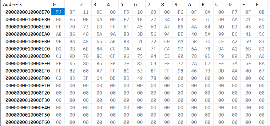
Figure 6. Compressed Data of an 8*8 Tile

5. Test results

Table 1. Compression Ratio of Test Images

6. Conclusion

This paper proposes a multi-predictor-based ARGB lossless texture compression algorithm. To facilitate hardware implementation, integer adaptive arithmetic coding is employed, achieving high compression ratios under low complexity. Consistency between software implementation and hardware verification validates the correctness and effectiveness of the algorithm, providing new insights for further research in the field of lossless image compression.

References

[1]. Yin, M., & Sun, G. (2024). FPGA design of a lossless ARGB data compression and decompression algorithm. Computer Measurement & Control, 32(02), 317-324. https://doi.org/10.16526/j.cnki.11-4762/tp.2024.02.045
[2]. Chen, D., Yu, M., Dai, M., et al. (2020). Lossless image compression of acyclic graphs based on variable bit-rate coding. Control Engineering, 27(05), 812-818. https://doi.org/10.14107/j.cnki.kzgc.20190452
[3]. Jiang, H., & Zhou, X. (2003). Lossless image compression based on local texture features. Journal of Beijing University of Aeronautics and Astronautics, (06), 505-508. https://doi.org/10.13700/j.bh.1001-5965.2003.06.009
[4]. Weinberger, M. J., Seroussi, G., & Sapiro, G. (2000). The LOCO-I lossless image compression algorithm: principles and standardization into JPEG-LS. IEEE Transactions on Image Processing, 9(8), 1209-1224.
[5]. Sheikh, H. R., Bovik, A. C., & Cormack, L. (2005). No-reference quality assessment using natural scene statistics: JPEG2000. IEEE Transactions on Image Processing, 14(11), 1918-1927.
[6]. Wu, X., & Memon, N. (2000). Context-based lossless interband compression--extending CALIC. IEEE Transactions on Image Processing, 9(6), 994-1001.
[7]. Wu, X. (1997). Lossless compression of continuous-tone images via context selection, quantization, and modeling. IEEE Transactions on Image Processing, 6(5), 656-664.
[8]. Wu, X. (2017). Research on arithmetic coding algorithm in image compression. Computer and Digital Engineering, 45(09), 1863-1865.
[9]. Wang, C., & Wang, J. (2004). Data compression method based on energy threshold and adaptive arithmetic coding. Power System Automation, (24), 56-60.
Cite this article
Mo,H. (2024). A multi-predictor based lossless ARGB texture compression algorithm and FPGA implementation. Advances in Engineering Innovation,9,62-68.
Data availability
The datasets used and/or analyzed during the current study will be available from the authors upon reasonable request.
Disclaimer/Publisher's Note
The statements, opinions and data contained in all publications are solely those of the individual author(s) and contributor(s) and not of EWA Publishing and/or the editor(s). EWA Publishing and/or the editor(s) disclaim responsibility for any injury to people or property resulting from any ideas, methods, instructions or products referred to in the content.
About volume
Journal:Advances in Engineering Innovation
© 2024 by the author(s). Licensee EWA Publishing, Oxford, UK. This article is an open access article distributed under the terms and
conditions of the Creative Commons Attribution (CC BY) license. Authors who
publish this series agree to the following terms:
1. Authors retain copyright and grant the series right of first publication with the work simultaneously licensed under a Creative Commons
Attribution License that allows others to share the work with an acknowledgment of the work's authorship and initial publication in this
series.
2. Authors are able to enter into separate, additional contractual arrangements for the non-exclusive distribution of the series's published
version of the work (e.g., post it to an institutional repository or publish it in a book), with an acknowledgment of its initial
publication in this series.
3. Authors are permitted and encouraged to post their work online (e.g., in institutional repositories or on their website) prior to and
during the submission process, as it can lead to productive exchanges, as well as earlier and greater citation of published work (See
Open access policy for details).