1. Introduction

Landscape driving forces can be defined as various factors and processes that influence and shape landscape change [1]. These forces may be natural, such as climate, landform, and hydrological processes, or anthropogenic, such as urbanization, agricultural expansion, road construction, and mining activities [2]. To explore the mechanisms driving landscape change, it is first necessary to identify the main driving factors and then examine their complex relationships with landscape pattern evolution. The complexity and uncertainty inherent in urban development are major contributors to changes in urban landscape patterns, permeating the entire process of urban ecosystem evolution and influencing both landscape patterns and processes. Therefore, it is essential to comprehensively consider the interactions among driving factors [3].

Since the 1960s, researchers in the field of landscape ecology have begun to explore the influence of natural factors on landscape change, including fire, floods, and wind erosion. In the 1980s, research expanded to include human activities, with a focus on agriculture and urbanization. Turner et al. proposed the “Pressure-State-Response (PSR)” model [4]. In the 21st century, American ecologist Jianguo Wu introduced the “landscape transformation framework,” which systematically analyzes landscape changes across different scales, speeds, and intensities, as well as their impacts on human well-being [5]. Koomen analyzed land use and temporal driving forces in European rural areas [6]; Hersperger et al. studied the driving forces of landscape change during urbanization [7]; Aimes applied weighted regression to analyze forest landscape evolution in the State of Mexico [8]. At present, research on landscape driving forces has evolved into a series of quantitative analyses of driving factors. Gong Yingbi analyzed the driving mechanisms behind the spatial-temporal evolution of urban wetland landscape patterns in Changsha [9]; Fu Hongyan conducted a study on the evolution and driving forces of landscape patterns in Nanchang [10]; Hu Juan et al. analyzed the evolution and driving forces of wetland landscape patterns in the Ziya River Basin from 2000 to 2014 [11]; Luo Yunjian quantitatively studied the spatial-temporal evolution characteristics and driving mechanisms of urban construction land expansion in Yangzhou [12]; Che Tong et al. examined the characteristics and driving forces of landscape pattern changes in construction land during urban expansion [13]; Dong Yuhong et al., based on GIS technology, analyzed the changes in landscape patterns and their driving forces in Taocheng District of Hengshui City [14].

Landscape driving forces represent the comprehensive forces behind changes in landscape types. At small spatial and temporal scales, relatively stable natural factors play a constraining role in landscape pattern changes, while frequently changing socioeconomic drivers are the direct forces driving such changes. Research on landscape driving forces is problem-oriented and lacks a fixed methodology. Considering the short temporal scale of this study and the substantial influence of socioeconomic factors on landscape pattern change, a combined quantitative and qualitative approach is adopted for analysis. This study selects natural, demographic, economic development, and social policy factors affecting the landscape pattern of the study area. Through dimensionality reduction using PCA, key factors are extracted to reveal the causes of landscape pattern changes in the study area.

City S is located in the south-central part of Hebei Province, China, between 37°27’–38°47’ N and 113°30’–115°20’ E [15], and is one of the core cities in the Beijing-Tianjin-Hebei urban agglomeration, with a total administrative area of 14,530 km².

2. Research content

Based on statistical yearbook data for City S from 2013 to 2020 [16], this study selected 28 driving force indicators across four major categories—natural factors, demographic factors, economic development factors, and social policy factors—for analysis. These indicators include: annual average temperature, annual precipitation, resident population, non-agricultural population, agricultural population, gross regional product, gross output value of agriculture, forestry, animal husbandry, and fishery, the composition of the primary, secondary, and tertiary industries, total industrial output value above designated size (in 100 million RMB), profits of industries above designated size, actual utilization of foreign capital, total import and export value, general public budget revenue, fixed asset investment, total retail sales of consumer goods, disposable income of urban residents, disposable income of rural residents, consumption level of urban residents, consumption level of rural residents, grain output, cultivated land area, highway mileage, afforested land area, number of domestic tourists, number of people covered by the minimum living standard guarantee system, and number of health institutions.

The interactions among demographic, economic development, and social policy factors are particularly prominent, making their impact on landscape patterns more complex. The total resident population reflects, to some extent, the scale of the city, while the numbers of agricultural and non-agricultural populations indicate the level of urbanization and the scale of agricultural development. Gross Regional Product (GDP) represents the overall economic performance of the area; the gross output value of agriculture, forestry, animal husbandry, and fishery reflects the scale and results of agricultural production over a given period. The composition of the primary, secondary, and tertiary industries reveals the structure of the economy, where sectors like real estate and design in the tertiary industry rapidly reshape urban landscapes through efficient construction activities. The transformation of the secondary industry and the rapid development of the real estate sector have promoted changes in regional landscape patterns. The total industrial output value and profits of industries above designated size reflect the scale and outcomes of industrial production during a certain period. The actual utilization of foreign capital indicates the extent of economic development supported by external investment, while total import and export value represents the overall volume of foreign trade. General public budget revenue and fixed asset investment reflect the state’s financial participation in social product distribution and serve as a financial guarantee for fulfilling government functions. Indicators such as total retail sales of consumer goods, disposable income of urban and rural residents, and their consumption levels reflect the income and consumption scales of urban dwellers. Grain output and cultivated land area indicate the state of agricultural development, which is influenced by temperature and precipitation and, in turn, affects rural residents’ disposable income. Indicators such as highway mileage, afforested land area, the number of people receiving minimum living standard subsidies, and the number of health institutions reflect the living conditions of urban residents. Improvements in urban infrastructure and services have accelerated the urbanization process. The enhancement of road and transport infrastructure promotes urbanization along traffic corridors and acts as a major driver of the urbanization process. Increases in the mileage of urban roads, highways, and rail transit systems, along with the development of large-scale urban transportation networks, often lead to a grid-like urban landscape and contribute to greater landscape fragmentation. The number of domestic tourists reflects tourism development, which affects scenic area planning and landscape construction.

Among the 28 selected indicators, varying degrees of correlation were observed. Some are positively correlated—for instance, resident population and gross regional product show a correlation coefficient of 0.463—while others are negatively correlated, such as gross regional product and total industrial output value above designated size. These 28 indicators influence one another and jointly shape the landscape pattern.

The contribution rates of the first three principal components are 64.359%, 17.669%, and 8.300%, respectively, with a cumulative contribution rate of 90.328%, meeting the required threshold. Therefore, the first three principal components can be used to replace the original 28 indicators, effectively reflecting the vast majority of information in the dataset. The rotated component matrix of the principal component analysis displays the correlations of indicators within each principal component. Subsequently, the principal component score coefficient matrix was calculated, which was then used to compute the annual scores and composite scores for each year (see Tables 1–5).

Table 1. Statistical data of selected factors 2013- 2020 in Shijiazhuang metropolitan area

Table 2. Driver indicator correlation

Table 3. The driver indicator eigenvalues and contribution rate of driving force factors

Table 4. The rotation matrix of principal components

Table 5. Component score coefficient matrix

3. Research results

A comprehensive principal component model was calculated using the proportion of each principal component’s eigenvalue to the total eigenvalue of all extracted principal components as weights. The F values were then calculated, as shown in Table 6.

Table 6. Principal component analysis and comprehensive evaluation results by each year

The trend of the F value is illustrated in Figure 1. From 2013 to 2020, except for a slight decline in a few individual years, the comprehensive value F of the driving force analysis model showed an overall upward trend. This indicates that the influence of the three principal components on the landscape pattern has generally increased year by year.

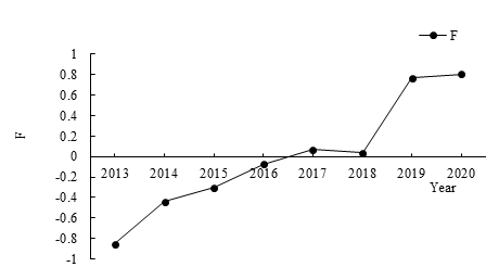
Figure 1. Changes of F value

An analysis of the three principal components reveals the following: The first principal component is mainly negatively correlated with the share of primary industry and the minimum living security coverage for urban and rural residents, and positively correlated with fixed asset investment, total retail sales of consumer goods, highway mileage, and the number of domestic tourists. The second principal component is primarily negatively correlated with the total output value of agriculture, forestry, animal husbandry, and fishery, as well as the total import and export value. It is positively correlated with the agricultural population, grain output, and cultivated land area. The third principal component is only negatively correlated with annual precipitation. In summary, four types of factors—natural factors, population factors, economic development factors, and social policy factors—serve as driving forces behind changes in landscape patterns.

Natural, population, economic development, and social policy factors collectively influence urban landscape patterns, interacting with and affecting one another. As cities are regions of intensive human activity, the influence of natural factors on urban landscape patterns is lower than their impact on natural habitat patterns. Over a ten-year timeframe, geological changes and wind direction have limited influence on the landscape pattern of the main urban area of S City, which is located in a plain region. The main driving factors are precipitation and temperature, which affect vegetation and the urban thermal environment.

References

[1]. Bürgi, M., Hersperger, A. M., & Schneeberger, N. (2004). Driving forces of landscape change: Current and new directions. Landscape Ecology, 19(8), 857–868.
[2]. Wei, W., Zhang, Y. L., Zhao, B., & Wang, H. (2011). The impact of urban expansion on landscape pattern differentiation during rapid urbanization. Ecology and Environmental Sciences, 20(1), 7–12.
[3]. Xiao, Y., Wang, Y. H., & Yin, C. (2010). Study on land use change in Beijing’s urban area over the past 20 years based on TM imagery. In Chinese Society of Remote Sensing (Ed.), Proceedings of the 17th China Remote Sensing Conference (p. 201).
[4]. Li, G. D., & Qi, W. (2019). The impact of construction land expansion on the evolution of landscape patterns in China. Acta Geographica Sinica, 74(12), 2572–2591.
[5]. Li, C., Li, J. X., & Wu, J. G. (2018). What drives urban growth in China? A multi-scale comparative analysis. Applied Geography, 98, 43–51.
[6]. Koomen, E., Bakema, A., Stillwell, J., & Scholten, H. (1999). Land-use changes and their environmental impact in rural areas in Europe. In UNESCO Reports (pp. 81–102). Paris: UNESCO.
[7]. Hersperger, A. M., & Bürgi, M. (2007). Driving forces of landscape change in the urbanizing Limmat Valley, Switzerland. In Koomen, E., Stillwell, J., Bakema, A., & Scholten, H. (Eds.), Modelling Land-Use Change (pp. 45–60). Springer.
[8]. Aimes, N. B. P., Sendra, J. B., & Delgado, M. G. (2010). Exploring the driving forces behind deforestation in the State of Mexico using geographically weighted regression. Applied Geography, 30(4), 576–591.
[9]. Gong, Y. B. (2013). Research on the spatial-temporal evolution and driving mechanism of urban wetland landscape pattern in Changsha [Master’s thesis, Central South University of Forestry and Technology].
[10]. Fu, H. Y. (2014). Study on urban landscape pattern evolution and driving forces in Nanchang City [Master’s thesis, East China University of Technology].
[11]. Hu, J., Ma, A. Q., & Ma, B. R. (2017). Wetland landscape pattern evolution and driving force analysis in the Ziya River Basin from 2000 to 2014. Journal of Ocean University of China, 47(9), 110–118.
[12]. Luo, Y. J., & Li, C. (2019). Spatiotemporal evolution and driving mechanism of construction land expansion in Yangzhou. Chinese Journal of Ecology, 38(6), 1872–1880.
[13]. Che, T., Li, C., & Luo, Y. J. (2020). Landscape pattern evolution and its driving forces of construction land during urban expansion. Acta Ecologica Sinica, 40(10), 3283–3294.
[14]. Dong, Y. H., Wu, D. Y., Wang, Y., & Sun, S. W. (2022). Landscape pattern change and its driving forces in Taocheng District, Hengshui City based on GIS. Hubei Agricultural Sciences, 61(21), 45–49, 129.
[15]. Li, Y. Y. (2021). Research on spatial structure of the ecological urban agglomeration in the Beijing-Tianjin-Hebei region [Master’s thesis, Beijing Jiaotong University].
[16]. Shijiazhuang Bureau of Statistics. (n.d.). Statistical Bulletin on National Economic and Social Development of Shijiazhuang. Retrieved May 12, 2025, from https://tjj.sjz.gov.cn/columns/7de8ce3b-2c70-4ea5-a3eb-e084223b5c52/index.html
Cite this article
Zhang,Y.;Wang,Z. (2025). Analysis of urban landscape change driving forces based on principal component analysis: a case study of City S in North China. Advances in Engineering Innovation,16(6),1-9.
Data availability
The datasets used and/or analyzed during the current study will be available from the authors upon reasonable request.
Disclaimer/Publisher's Note
The statements, opinions and data contained in all publications are solely those of the individual author(s) and contributor(s) and not of EWA Publishing and/or the editor(s). EWA Publishing and/or the editor(s) disclaim responsibility for any injury to people or property resulting from any ideas, methods, instructions or products referred to in the content.
About volume
Journal:Advances in Engineering Innovation
© 2024 by the author(s). Licensee EWA Publishing, Oxford, UK. This article is an open access article distributed under the terms and
conditions of the Creative Commons Attribution (CC BY) license. Authors who
publish this series agree to the following terms:
1. Authors retain copyright and grant the series right of first publication with the work simultaneously licensed under a Creative Commons
Attribution License that allows others to share the work with an acknowledgment of the work's authorship and initial publication in this
series.
2. Authors are able to enter into separate, additional contractual arrangements for the non-exclusive distribution of the series's published
version of the work (e.g., post it to an institutional repository or publish it in a book), with an acknowledgment of its initial
publication in this series.
3. Authors are permitted and encouraged to post their work online (e.g., in institutional repositories or on their website) prior to and
during the submission process, as it can lead to productive exchanges, as well as earlier and greater citation of published work (See
Open access policy for details).