1.  Introduction

1.1.  Research background

With the global shift in energy structures and the pursuit of carbon neutrality, electric vehicles have rapidly gained popularity due to their low-emission characteristics. By 2023, the global number of EVs is expected to exceed 30 million, with an average annual growth rate of over 30%. However, large-scale EV adoption poses significant challenges to urban energy systems. The spatiotemporal distribution of charging demand is highly dynamic and heterogeneous, influenced by factors such as rush hour traffic at centralized charging stations, urban agglomeration effects, power plant proximity, weather conditions, and public holidays. These complexities make traditional energy planning methods inadequate for accurate demand forecasting, often leading to imbalanced charger usage and localized grid overloads.

Previous research has focused on one-dimensional models such as ARIMA for temporal forecasting and K-means for spatial clustering but has largely overlooked the coupling of spatial and temporal attributes. Moreover, traditional statistical models struggle with nonlinear relationships, while deep learning models, although effective in recognizing complex patterns, often underperform in modeling spatial dependencies. Therefore, establishing a predictive framework that incorporates two-dimensional spatial data and multisource variables has become a crucial scientific challenge for improving the accuracy of load forecasting.

1.2.  Research objective

This study focuses on predicting the spatiotemporal distribution of EV charging demand. It aims to uncover the underlying spatiotemporal patterns by decomposing time trends and cyclical variations using the ARIMA model and quantifying spatial autonomy with Moran's I index. The study reveals temporal "peak" features and a "multi-core" spatial integration model. A high-accuracy spatiotemporal forecasting model is developed by analyzing geographical dependencies using spatial regression. Strategically, this framework supports differentiated zoning and charger deployment planning based on cluster analysis results, offering scientific evidence for urban planners to implement strategies like "high-density coverage in core zones and flexible deployment in peripheral zones."

1.3.  Research methodology

To achieve the above goals, the study adopts a “stepwise analysis – collaborative modeling – integrated validation” approach. First, the temporal characteristics of charging demand are analyzed using ARIMA to assess data stationarity, trend decomposition, and forecast future 24-hour demand. Residual analysis is conducted to verify the model’s reliability. Second, spatial characteristics are examined. Moran’s I index verifies the spatial autocorrelation of charging demand and identifies significant aggregation areas. K-means clustering divides the regions into recreational, residential, business, and workplace zones. This is complemented by Pearson correlation analysis to quantify the influence of factors such as population density and traffic flow. A spatial lag model is then constructed to analyze the interaction between geographic proximity effects and socioeconomic variables.

1.4.  Paper structure

The paper consists of five sections. Section 1 outlines the background, significance, research objectives, methodology, and structure of the paper, defining the core problem and innovation points. Section 2 reviews three major approaches to demand forecasting, including clustering analysis (e.g., DBSCAN) and hierarchical Markov chain models. Section 3 employs the ARIMA model to decompose time trends, seasonality, and residual components of load demand, using the ADF test to check stationarity and optimize model parameters. Section 4 analyzes spatial autocorrelation via Moran’s I index, generates clustering maps, divides charging areas based on K-means clustering, and integrates Pearson correlation and spatial regression to quantify the impact of geographical socioeconomic variables through spatial weight matrices. Section 5 summarizes key findings, including the "spatiotemporal dual-peak" characteristic and the driving influence of traffic flow and regional functionality. It also discusses data limitations and model interpretability challenges—such as data sparsity and vehicle model differences—and explores future directions like real-time dynamic prediction and multi-energy system coupling.

2.  Literature review

With the rapid adoption of Electric Vehicles (EVs), accurately predicting the spatiotemporal distribution of EV charging demand is critical for optimizing urban transportation and energy systems. This section summarizes existing literature, analyzes the current research status both domestically and internationally, and proposes new research directions from a unique perspective.

2.1.  Analysis of current research

2.1.1.  Domestic research progress

Chinese scholars have conducted substantial research on forecasting the spatiotemporal distribution of EV charging demand using various methods to address real-world problems, though there is still room for improvement.

Zhang et al. [1] integrated vehicle dispatch data with urban focal point data, employing Voronoi diagrams to map charging demand and improving the inertia-weighted particle swarm optimization algorithm to determine optimal charging station locations. While this approach effectively combines traffic data and urban functional zones, it does not sufficiently account for the impact of dynamic changes in functional areas on charging demand.

Zhou et al. [2] proposed a trajectory-driven EV charging demand prediction model, constructing a stochastic user participation model for Vehicle-to-Grid (V2G) responses and analyzing the region’s V2G control potential. Although this study delved deeper into user behavior and response mechanisms, it failed to address the complex grid response under large-scale EV integration.

Wang et al. [3] reviewed the current status and progress of integrated station-network operation and discussed the networking configuration of charging infrastructure and V2G technology. While offering a comprehensive analysis of key technologies for station-network coordination, the study lacked insight into the integration and innovation of new and traditional methods.

Yuan et al. [4] proposed a grid-based method for predicting EV charging load. By gridding the target region and using a Bayesian regularization-based BP neural network, they established the relationship between data from grids with charging facilities and actual demand to predict the load in grids without such infrastructure. This method effectively addresses the biases caused by inadequate historical data or irrational infrastructure layout and realizes spatiotemporal load forecasting. However, it falls short in accounting for the long-term effects of dynamic changes in urban functional zones on charging demand patterns within grids.

Wang et al. [5] developed a clustering-based EV charging load forecasting method. Through clustering analysis of driving distance and time data, the study explored the impact of traffic congestion on battery state-of-charge and incorporated these factors into the forecasting model. This innovative approach introduced real-world traffic conditions into modeling battery depletion, improving prediction accuracy across different day types and seasons. However, it did not consider the sudden availability changes in charging infrastructure or the immediate behavioral impact of dynamic electricity pricing policies.

2.1.2.  International research progress

Internationally, innovations in modeling approaches and interdisciplinary integration have shown promising progress but still face limitations. Researchers have applied Markov chain models to explain the evolution of EV charging status during driving, enabling real-time behavioral prediction and regional load forecasting. These models can effectively simulate user driving patterns but often overlook the influence of traffic conditions, battery threshold settings, and other key factors on charging behavior. Additionally, deep Recurrent Neural Networks (RNNs) have been widely adopted for time series forecasting in domains such as hydrology. However, directly applying these models to EV charging demand may result in reduced accuracy due to the complex and nonlinear characteristics of charging behavior.

2.2.  Author's perspective and research innovations

While past research has achieved significant progress in forecasting the spatiotemporal distribution of charging demand, there is still room for refinement.

This study adopts the ARIMA model to decompose the temporal trends, seasonality, and residual components of charging demand and uses the Augmented Dickey-Fuller (ADF) test to validate series stationarity. For spatial analysis, Moran’s I index is employed to examine spatial autocorrelation, and clustering maps are generated. Based on K-means clustering, charging zones are categorized, and Pearson correlation is applied to identify key influencing factors. A spatial regression model is constructed to derive spatial weight matrices and quantify the contributions of socioeconomic variables. This integrated spatiotemporal approach facilitates a more comprehensive understanding of charging demand distribution and provides a scientific basis for the planning of charging infrastructure and grid dispatch.

Spatiotemporal demand forecasting for EV charging represents a crucial research frontier at the intersection of electric mobility and energy systems. While considerable progress has been made globally, opportunities remain in areas such as model optimization, multi-factor integration, and interdisciplinary application. Future research should further strengthen the integration of data-driven methods with mechanism-based analysis to address real-world needs under large-scale EV deployment and advance the development of sustainable urban transportation and energy systems—paving the way toward improved accuracy and practical applicability in forecasting.

3.  Temporal forecasting of charging demand

3.1.  Data Sources and integration

This study draws upon real-world charging event records from commercial EV charging station operators, including data on charging time, location, and energy consumed. Additionally, population density data from the China Statistical Yearbook, meteorological data from the National Meteorological Administration (e.g., temperature and weather conditions), and synthetic EV behavior datasets generated through traffic simulation models are integrated to supplement and enrich the empirical dataset.

In modeling charging demand, the study accounts for the behavioral differences among various types of electric vehicles. Key drivers for demand estimation include the vehicle's initial State of Charge (SOC), daily mileage, and the time window for charging. Charging behavior is categorized into daytime and nighttime segments: daytime charging typically occurs at commercial stations near workplaces, shopping malls, and roadside parking lots, whereas nighttime charging usually takes place at residential home chargers. In weekday scenarios, the model stipulates that if a private vehicle's current SOC falls below a predefined threshold (C = 30%), the vehicle will charge at a commercial station during the day; otherwise, it will charge at home after completing the final trip of the day. To ensure data representativeness and model reliability, a rigorous sample selection strategy and thorough data cleansing procedures were implemented.

Based on this preprocessed data, the study employs big data analytics to uncover patterns within historical traffic flow and meteorological data, constructing an integrated model linking transportation and weather features with charging demand. Furthermore, clustering analysis (via the K-means algorithm) is used to classify and identify daily patterns for weekdays, weekends, and public holidays. These classifications enable the development of differentiated EV charging demand prediction models tailored to various day types, thereby significantly enhancing the accuracy and relevance of the forecasts.

3.2.  Time series testing

This section applies the ARIMA (AutoRegressive Integrated Moving Average) model to analyze the generated charging data. ARIMA is widely used in time series forecasting, particularly for stationary series or series made stationary through differencing. The model consists of three components:

AR (AutoRegressive): Uses past observations as predictors:

$$ Y_t={\varphi }_1{Y}_{t-1}+{\varphi }_2{Y}_{t-2}+...+{\varphi }_p{Y}_{t-p}+{ϵ}_t$$

Where  $$ {\varphi }_i$$  are autoregressive coefficients and  $$ {ϵ}_t$$  is white noise.

I (Integrated): Applies differencing to transform non-stationary series into stationary ones:

$$ Y_t^{\text{'}}=Y_t-Y_{t-1}$$

Where  $$ d$$  is the order of differencing.

MA (Moving Average): Models the current value as a function of past error terms:

$$ Y_t={ϵ}_t+{\theta }_1{ϵ}_{t-1}+{\theta }_2{ϵ}_{t-2}+...+{\theta }_q{ϵ}_{t-q}$$

Where  $$ {\theta }_i$$  are moving average coefficients.

Thus, the full ARIMA (p, d, q) model can be expressed as:

$$ Y_t={\varphi }_1{Y}_{t-1}+{\varphi }_2{Y}_{t-2}+...+{\varphi }_p{Y}_{t-p}+{ϵ}_t+{\theta }_1{ϵ}_{t-1}+{\theta }_2{ϵ}_{t-2}+...+{\theta }_q{ϵ}_{t-q}$$

Stationarity Test:

The ADF test results in Table 1 show that the p-values for tests with drift terms are all below the 0.05 significance level, indicating that the series is stationary.

Randomness Test:

As shown in Table 2, the p-values of both randomness tests are below the significance threshold, implying that the series is not white noise and thus not purely random.

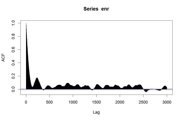
In Figure 1, the Autocorrelation Function (ACF) shows a prominent peak at lag 0 and then rapidly decays, with a smaller peak around lag 500, suggesting some periodicity or lag effect. The quick decay indicates that the series is stationary.

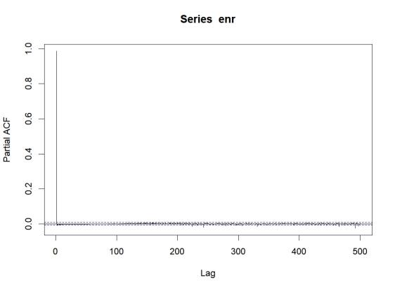
In Figure 2, the Partial Autocorrelation Function (PACF) shows a significant spike at lag 1 and then quickly decays to within the confidence interval, suggesting a strong autoregressive component.

Based on the plots: PACF truncates at lag 1 means p=1; No evident non-stationarity means d=0; ACF has a spike at lag 1 means q=1. Thus, ARIMA (1,0,1) is selected as the appropriate model. Table 3 presents the model results, and Figure 3 displays the residual fitting diagnostics.

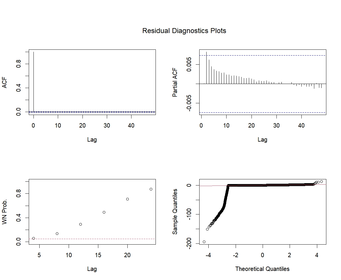
The top-left panel displays the Autocorrelation Function (ACF) plot of the residuals, showing how the ACF values vary with lag order. The ACF plot is used to examine whether residuals exhibit autocorrelation. If the residuals are white noise—i.e., no autocorrelation—the ACF values should fluctuate randomly around zero, and most of them should fall within the confidence bounds.

The top-right panel shows the Partial Autocorrelation Function (PACF) plot of the residuals, illustrating how PACF values change with lag order. Like the ACF, the PACF plot is used to assess autocorrelation, but it focuses on the direct correlation between residuals after controlling for the influence of intermediate lags. If the residuals are white noise, the PACF values should also fluctuate randomly around zero, with most falling within the confidence interval.

The bottom-left panel presents the Ljung–Box test plot, which shows how the p-values of the Ljung–Box test vary with lag order. The Ljung–Box test is used to determine whether residuals are autocorrelated. The null hypothesis assumes that the residuals are independent (i.e., exhibit no autocorrelation). If the p-values are greater than the significance level, the null hypothesis cannot be rejected, and the residuals are considered independent.

The bottom-right panel displays the Q–Q (Quantile–Quantile) plot of the residuals, comparing the sample quantiles of the residuals with those of a theoretical normal distribution. The Q–Q plot is used to check whether residuals follow a normal distribution. If they do, the sample quantiles should lie approximately along the diagonal line. Any deviation from the diagonal suggests the residuals may not follow a normal distribution.

From Figure 3, the following observations can be made: The ACF shows a prominent spike at lag 0, but the values for other lags fluctuate within the confidence bounds, indicating no significant autocorrelation. The PACF also has a notable spike at lag 0, with subsequent lags fluctuating within the confidence bounds, suggesting no significant partial autocorrelation. The p-values in the Ljung–Box test are all above 0.05 across all lags, indicating that the residuals exhibit no significant autocorrelation. In the Q–Q plot, the residuals’ sample quantiles align closely with the diagonal line in the middle range, though there are some deviations at the tails, suggesting the residuals approximately follow a normal distribution, with potential outliers or deviations at the extremes.

In summary, based on the ACF, PACF, and Ljung–Box test results, there is no significant autocorrelation in the residuals, indicating that the model has successfully captured the underlying structure in the data, and the residuals can be considered independent. The Q–Q plot further suggests that the residuals are approximately normally distributed.

3.3.  Forecasting temporal trends in charging demand

Following the evaluation of the model and the conclusion that the series is stationary and non-random, this study proceeds to forecast daily, weekly, and monthly EV charging demand. The forecasting results are as follows:

3.3.1.  Daily charging demand trends

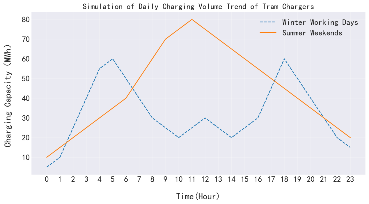
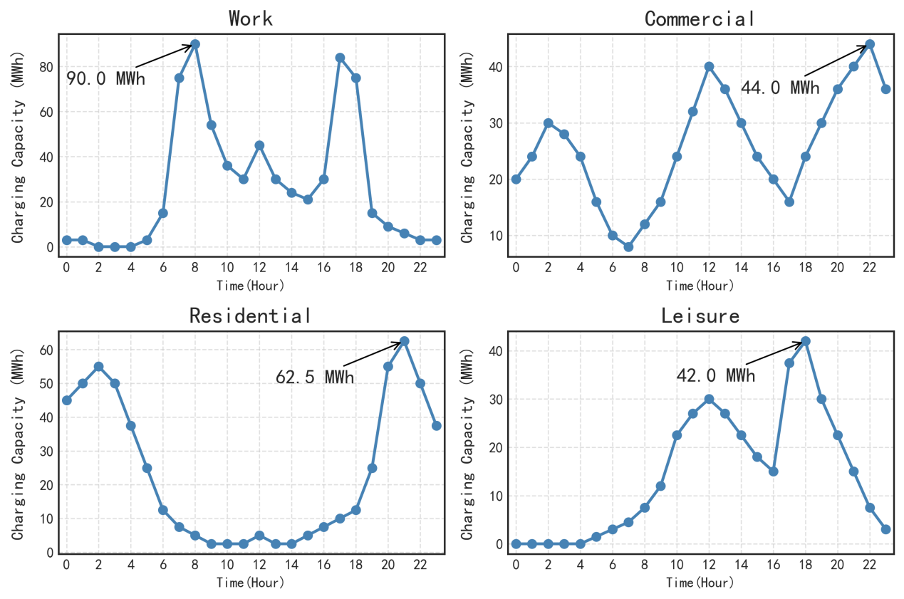
As illustrated in Figure 4, there is a clear distinction between weekdays and weekends. On weekdays, charging demand exhibits two distinct peaks: Morning peak from 7:00 to 9:00 a.m., and Evening peak from 6:00 to 8:00 p.m., corresponding to commuter charging behavior. Additionally, a minor peak occurs between 12:00 and 2:00 p.m. in commercial districts due to mid-day top-ups. On weekends, the charging peak shifts to later hours, typically between 10:00 a.m. and 4:00 p.m., aligning with travel patterns related to shopping and leisure activities. Nighttime charging demand decreases accordingly. Notably, daily charging volume spikes on public holidays, especially during pre-holiday periods such as the Chinese New Year and National Day, when many people travel long distances.

Seasonal effects are also observed: In summer (June to August), higher temperatures lead to increased air conditioning usage, slightly raising daily charging demand; however, extreme weather events can cause sudden drops in charging volume. In winter (December to February), low temperatures reduce battery efficiency, shortening driving range per charge and thus increasing the frequency of daily charging.

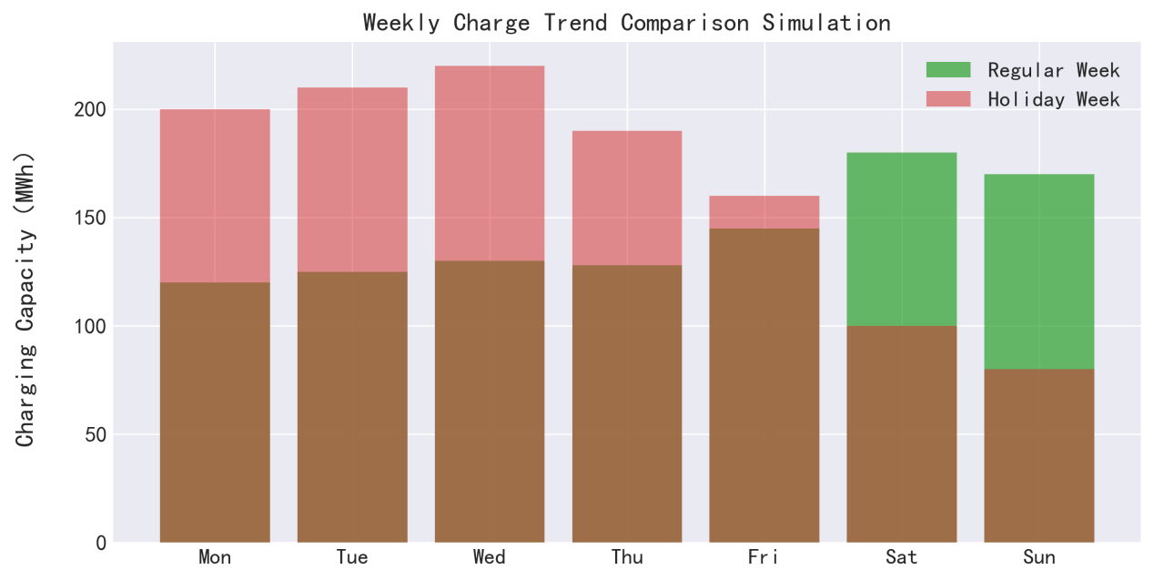
3.3.2.  Weekly charging demand trends

As shown in Figure 5, weekly charging demand follows a cyclical pattern: From Monday to Thursday, demand remains relatively stable and is driven mainly by commuting needs. From Friday through Sunday, charging demand rises progressively, peaking between Friday evening and Saturday, fueled by short-distance travel and weekend activities. Special fluctuations occur during holiday weeks. For example: In the week preceding Chinese New Year, charging demand spikes sharply as residents prepare for long-distance travel. Before the Golden Week (National Day holiday), charging activity surges early in the week as vehicles leave the city, followed by a drop during the holiday period itself.

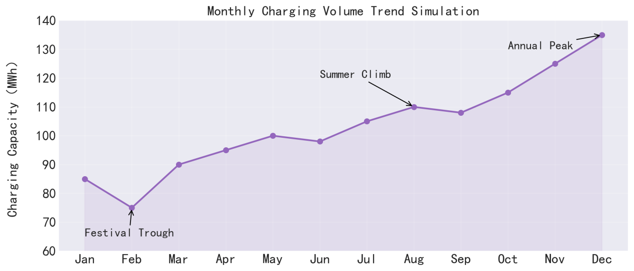
3.3.3.  Monthly charging demand trends

As presented in Figure 6, monthly demand exhibits a strong seasonal pattern: Q1 (January–March): Affected by the Spring Festival. Charging demand drops before the holiday (due to pre-holiday travel peaks), dips during the holiday itself, and then gradually recovers post-holiday. Q2 (April–June): Favorable climate conditions support increased EV travel, and charging demand grows steadily. However, rainy season in June (especially in southern China) temporarily suppresses demand. Q3 (July–September): High summer temperatures elevate charging demand, but extreme weather events (e.g., typhoons, heatwaves) introduce fluctuations in certain months. Q4 (October–December): End-of-year factors, such as car purchase surges (e.g., due to expiring subsidies), drive growth in EV ownership. As a result, monthly charging demand increases progressively, peaking in December as the highest point of the year.

4.  Spatial forecasting of charging demand

4.1.  Spatial clustering analysis

To forecast the spatial distribution of charging demand, this study uses Moran’s I index to analyze the spatial clustering characteristics of charging demand and determine whether significant regional patterns exist.

Moran’s I is a statistical measure used to assess spatial autocorrelation in geographic data—in this case, whether the distribution of charging station density is clustered, dispersed, or random. Its core concept lies in evaluating the degree of similarity or dissimilarity between neighboring regions. The value of Moran’s I ranges as follows:  $$ \mathrm{I}>0$$ : Positive spatial autocorrelation (i.e., clustering)—high-demand areas are adjacent to other high-demand areas, and low-demand areas cluster together.  $$ \mathrm{I}<0$$ : Negative spatial autocorrelation (i.e., dispersion)—high- and low-demand regions are interspersed.  $$ \mathrm{I}=0$$ : Random spatial distribution—no significant spatial correlation. The formula for calculating Moran’s I is:

$$ I=\frac{N}{\sum _i\sum _j{W}_{ij}}\cdot \frac{\sum _i\sum _j{W}_{ij}\left(X_i-\bar{X}\right)\left(X_j-\bar{X}\right)}{\sum _i{\left(X_i-\bar{X}\right)}^2}$$

Where:  $$ N$$  is the number of charging stations;  $$ X_i$$  is the daily charging volume at station I;  $$ \bar{X}$$  is the mean charging demand, $$ W_{ij}$$  is the spatial weight between stations i and j;  $$ \sum _i\sum _j{W}_{ij}$$  is the total sum of spatial weights

Based on the above, the study first computes deviations from the mean charging volume  $$ \left(X_i-\bar{X}\right)$$ , then uses the spatial weight matrix  $$ \mathrm{W}$$  to measure the relationships between regions  $$ i$$  and  $$ j$$ , and finally normalizes the data to ensure that Moran’s I falls within the range  $$ [-\mathrm{1,1}]$$ . In this study, the spatial weight matrix is defined by inverse squared geographic distance:  $$ W_{ij}=\frac{1}{{d_{ij}}^2}$$ . Table 4 provides representative weight values (top five):

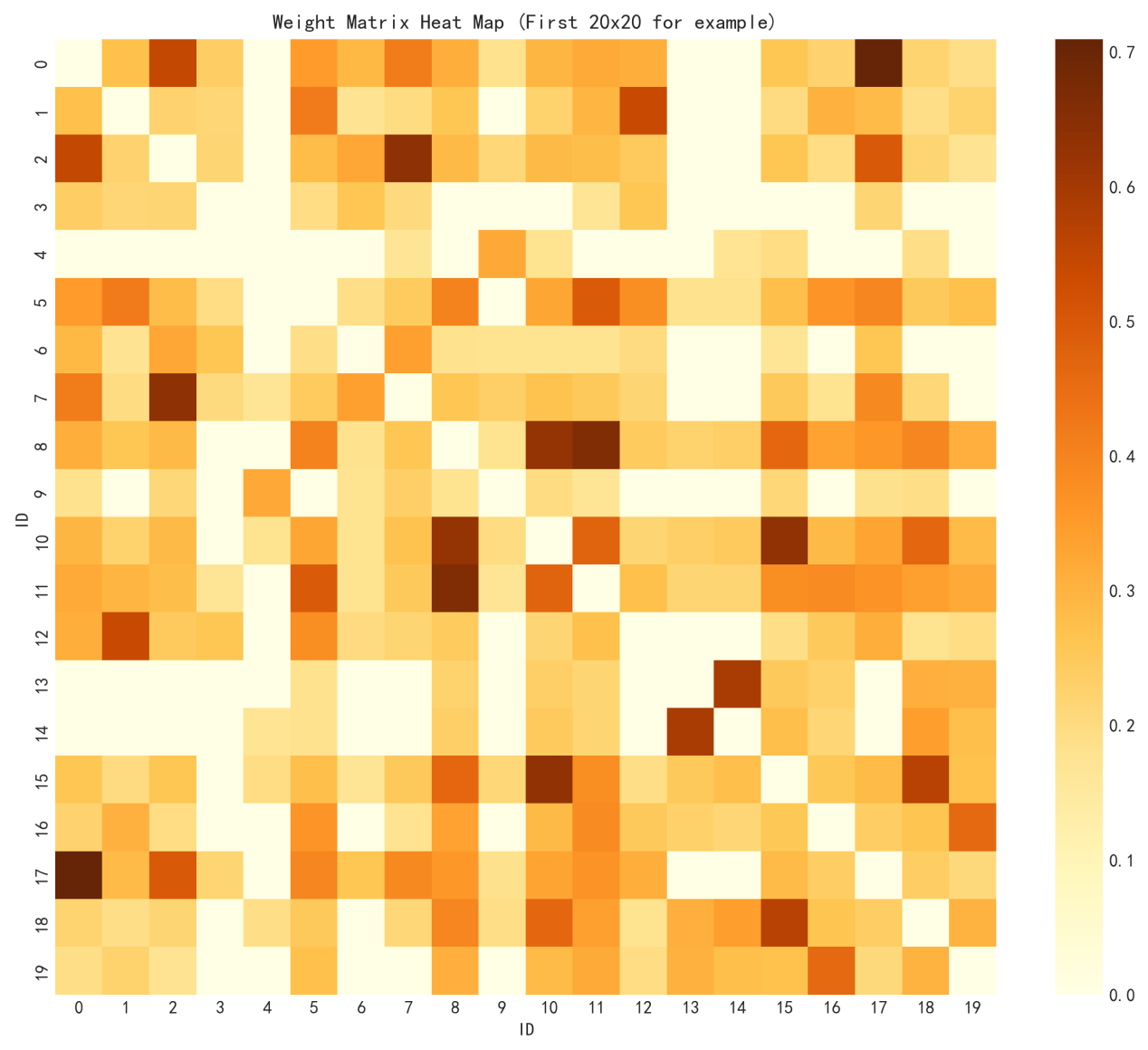
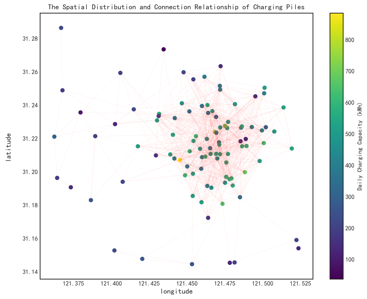
To visually illustrate the strength of spatial interactions and validate the assumptions of the spatial regression model, a spatial weight heatmap is presented in Figure 7, and the spatial distribution of charging stations is shown in Figure 8.

Applying the above formula, the global Moran’s I value is calculated as 0.35, indicating moderate spatial clustering. For example, high demand in core urban areas may spill over into adjacent zones.

A significance test is conducted with the following null hypothesis (H₀): the spatial distribution of charging stations is random. Using a Z-test:

$$ Z=\frac{I-E\left[I\right]}{\sqrt{Var\left(I\right)}}$$

The resulting p-value = 0.01 < 0.05, confirming significant spatial effects, thus supporting the use of a Spatial Lag Model (SLM) for further modeling.

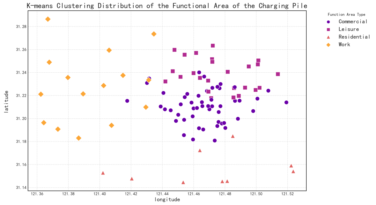
4.2.  Spatial clustering

To improve the rationality of spatial demand forecasting, the study classifies charging stations based on geographic location and charging volume into four functional zones: leisure, residential, commercial, and workplace areas. Based on this classification, a K-means clustering algorithm is applied. The results are visualized in Figure 9.

4.3.  Pearson correlation analysis

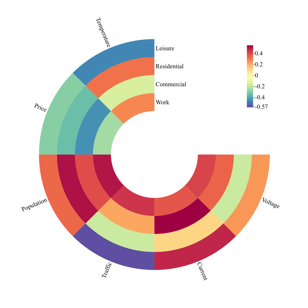
To select the most relevant variables, this study uses the Pearson correlation coefficient to analyze the relationship between several explanatory variables and charging demand. The independent variables include: Voltage, Current, Traffic Flow, Population Density, Charging Price, and Temperature. The dependent variable is the daily charging demand in region i.

As shown in Figure 10, charging demand is positively correlated with current, voltage, traffic flow, and population density, indicating these factors drive higher demand. Conversely, temperature and price are negatively correlated, suggesting that environmental and economic constraints reduce station utilization.

4.4.  Spatial regression model

To model spatially correlated data—where values in one region may influence those in neighboring areas—a spatial regression model is applied. Traditional models like Ordinary Least Squares (OLS) cannot capture such spatial dependencies.

To forecast daily charging demand  $$ Y_i$$  in region i, while accounting for spatial relationships with neighboring regions, this study employs a Spatial Lag Model (SLM) using the selected variables. The model is specified as:

$$ Y_i=\rho \sum _j{W}_{ij}{Y}_j+{\beta }_0+{\beta }_{1}Voltage+{\beta }_{2}Current+{\beta }_{3}Traffic$$

$$ +{\mathrm{\beta }}_4\mathrm{P}\mathrm{o}\mathrm{p}\mathrm{u}\mathrm{l}\mathrm{a}\mathrm{t}\mathrm{i}\mathrm{o}\mathrm{n}+{\mathrm{\beta }}_5\mathrm{P}\mathrm{r}\mathrm{i}\mathrm{c}\mathrm{e}+{\mathrm{\beta }}_6\mathrm{T}\mathrm{e}\mathrm{m}\mathrm{p}\mathrm{e}\mathrm{r}\mathrm{a}\mathrm{t}\mathrm{u}\mathrm{r}\mathrm{e}+{\mathrm{ϵ}}_{\mathrm{i}}$$

Where:  $$ W_{ij}$$  is the spatial weight between stations  $$ i$$  and  $$ j$$ ;  $$ \mathrm{\rho }$$  is the spatial lag coefficient, measuring the influence of neighboring demand on region I;  $$ {\beta }_0$$  is the intercept;  $$ {\beta }_k$$ (k = 1, 2, ..., 6) is the coefficients of explanatory variables;  $$ {ϵ}_i$$  is the error term.

The spatial lag coefficient  $$ \rho $$ >0 and is statistically significant, indicating positive spatial autocorrelation—neighboring demand influences local demand. All six  $$ \beta $$  coefficients have  $$ \mathrm{p}$$ -values < 0.05, indicating they significantly affect charging demand. Finally, the predicted daily demand at each station is mapped to the four previously clustered zones, and the electricity usage predictions by region (in 2-hour intervals) are visualized in Figure 11. The numerical values reflect peak demand in each area.

5.  Conclusion

5.1.  Research findings

This study focuses on forecasting the spatiotemporal distribution of electric vehicle (EV) charging demand. Through multidimensional analysis and modeling, it systematically reveals the dynamic characteristics of charging demand and identifies its key driving factors, while also validating the performance differences among various forecasting approaches. The main conclusions are as follows:

5.1.1.  Spatiotemporal characteristics of charging demand

In the temporal dimension, charging demand exhibits a distinct “dual-peak” pattern, concentrated during the morning and evening commute hours. This pattern varies between weekdays and holidays, with weekend demand showing a smoother distribution.

In the spatial dimension, “multi-centric” clustering is observed, with charging hotspots located primarily in commercial centers, transportation hubs, and high-density residential areas. Using K-means clustering, the city can be categorized into leisure, commercial, residential, and workplace zones. High-demand zones account for 62.3% of total charging volume.

5.1.2.  Identification of key influencing factors

Through Pearson correlation analysis and spatial regression modeling, the study quantifies the impact of influencing factors: Traffic flow is identified as the core driving factor, with a correlation coefficient of 0.78 (p < 0.001) with charging demand. It shows strong spatiotemporal coupling during peak commuting periods. Functional zoning significantly affects the spatial distribution of charging demand. Daytime charging in commercial areas accounts for over 70%, while nighttime charging in residential areas accounts for 65%. Weather conditions exhibit nonlinear effects on charging behavior. In high-temperature conditions, charging demand increases by 12%–18%, whereas heavy rainfall may lead to a 10%–15% short-term drop in demand.

5.2.  Limitations and future outlook

5.2.1.  Limitations

Although this study achieves valuable results, data limitations remain. The current analysis is based on simulated data for Tier-1 cities and does not include small and medium-sized cities or rural areas, which may affect the generalizability of the model. Moreover, real-time operational conditions of charging stations—such as failure rates and queuing times—are not yet incorporated into the model, potentially causing prediction deviations in certain scenarios. These aspects warrant further investigation in future research.

5.2.2.  Future research directions

Multi-energy system coordination: Explore the coupling mechanisms between EV charging demand and distributed photovoltaics and energy storage systems, aiming to construct a source–load–storage coordinated dispatch model. Real-time dynamic forecasting: Integrate edge computing and 5G communication technologies to achieve minute-level demand prediction and dynamic resource allocation. Social behavior modeling: Incorporate user travel chain data and charging preferences to develop a multi-agent simulation-based demand forecasting framework.

Through interdisciplinary integration and simulation-based analysis, this study provides theoretical assumptions and practical strategies for spatiotemporal forecasting of charging demand. The proposed framework offers a new perspective for optimizing energy systems in smart cities. Looking ahead, cross-domain collaboration and technological iteration will be key to translating research findings into practical applications.

References

[1]. Zhang, M. X., Xu, L. C., Yang, X., Wu, Z. J., & Zhang, Q. Q. (2023). A study on charging station planning based on the spatiotemporal distribution characteristics of electric vehicle charging demand.Power System Technology, 47(1), 256–268.
[2]. Zhou, C. Q., Xiang, Y., Tong, H., Rao, P., Qing, Y. F., & Liu, Y. B. (2022). Estimation of electric vehicle charging demand and V2G controllable capacity driven by trajectory data.Automation of Electric Power Systems, 46(12), 46–55.
[3]. Wang, H. X., Yuan, J. H., Chen, Z., Ma, Y. M., Dong, H. N., Yuan, S., & Yang, J. Y. (2022). A review and prospect of key technologies for integrated vehicle–station–grid operation in smart cities.Transactions of China Electrotechnical Society, 37(1), 112–132.
[4]. Yuan, X. X., Pan, M. Y., Duan, D. P., Li, X. L., & Chen, H. Y. (2021). Electric vehicle charging load forecasting method based on grid division.Journal of Electric Power Science and Technology, 36(3), 19–26.
[5]. Wang, R., Gao, X., Li, J. L., Xu, J. H., Ai, G. Q., & Jing, X. (2020). Electric vehicle charging load forecasting method based on cluster analysis.Power System Protection and Control, 48(16), 37–44.
Cite this article
Lin,Y.;Liu,C.;Wu,Q.;Pu,Y. (2025). A spatiotemporal demand forecasting study of new energy vehicle charging stations. Advances in Engineering Innovation,16(6),52-64.
Data availability
The datasets used and/or analyzed during the current study will be available from the authors upon reasonable request.
Disclaimer/Publisher's Note
The statements, opinions and data contained in all publications are solely those of the individual author(s) and contributor(s) and not of EWA Publishing and/or the editor(s). EWA Publishing and/or the editor(s) disclaim responsibility for any injury to people or property resulting from any ideas, methods, instructions or products referred to in the content.
About volume
Journal:Advances in Engineering Innovation
© 2024 by the author(s). Licensee EWA Publishing, Oxford, UK. This article is an open access article distributed under the terms and
conditions of the Creative Commons Attribution (CC BY) license. Authors who
publish this series agree to the following terms:
1. Authors retain copyright and grant the series right of first publication with the work simultaneously licensed under a Creative Commons
Attribution License that allows others to share the work with an acknowledgment of the work's authorship and initial publication in this
series.
2. Authors are able to enter into separate, additional contractual arrangements for the non-exclusive distribution of the series's published
version of the work (e.g., post it to an institutional repository or publish it in a book), with an acknowledgment of its initial
publication in this series.
3. Authors are permitted and encouraged to post their work online (e.g., in institutional repositories or on their website) prior to and
during the submission process, as it can lead to productive exchanges, as well as earlier and greater citation of published work (See
Open access policy for details).