1 Introduction

In a market economy, competition among firms is unavoidable. In order to gain a larger market share and profit, firms need to develop effective pricing strategies. In recent years, a concept from game theory called the prisoner's dilemma has attracted widespread attention. The prisoner's dilemma is a game theory model that describes the choices between cooperation and defection faced by two prisoners. This concept has been extensively studied in various fields, but its application in pricing strategies remains relatively limited. This dissertation aims to investigate the extent of the prisoner's dilemma's use in pricing strategies.

Pricing strategies play a significant role in determining the success and profitability of firms. Pricing too high may lead to a decrease in demand and customer loss, while pricing too low may result in reduced profitability. Therefore, setting the right price is a key factor in balancing payoff maximization and maintaining market competitiveness. In the context of pricing strategy, the prisoner's dilemma can provide valuable insights into the decision-making process of firms and the dynamics of competition.

With this in mind, primary goal of this paper emerges: The extent that the prisoner's dilemma be used in pricing strategies, and the effects of strategies taken by firms on their potential payoffs, the stability and sustainability of cooperative pricing agreement, limitations in using the prisoner's dilemma in pricing strategies. By examining the applicability of the prisoner's dilemma in pricing, we seek to shed light on the potential benefits and limitations of adopting this framework in real-world business scenarios.

In the rest of the papers, there will be a literature review part explaining concept of prisoner’s dilemma and related findings, common pricing strategies and the importance of prisoner’s dilemma in pricing. Then, there will be a discussion part about the application of prisoner’s dilemma to pricing. Finally, we summarize the extent of the application of the prisoner's dilemma in pricing strategies and propose future research directions.

2 Research review

2.1 Prisoner’s dilemma

2.1.1 Concept

The prisoner’s dilemma is a classic and famous game in non-cooperative game theory that illustrates how the self-interested actions of participants can result in an outcome that is less favorable for everyone involved. It is commonly used to analyse the possibility for cooperation in scenarios where individuals interact strategically with their own interests in mind.

The story of the prisoner's dilemma is as follows: Both suspects are arrested, and both of them are rational, self-interested, and unable to communicate with each other. They were told the following rules: Cooperate with their partner and remain silent, or betray each other, choose to defect. The prison sentences represent the payoffs of each decision and these payoffs of course depend on whether they accepts the deal offered and defects, or remains silent and cooperates. The following payoff matrix (Figure 1) describes the possible outcomes of the game.

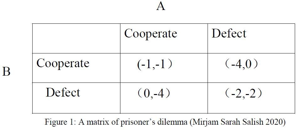
Figure 1. A matrix of prisoner’s dilemma [7]

What is the equilibrium of the game? The answer is that both people will choose to betray each other. From A's perspective, he thinks: If B remains silent and I choose to defect, I will be released immediately, instead of one year I would receive if B cooperates. If B defects me and I remain silent, I will be sentenced to four years in prison. So A will choose to defect. In the same way, B will also choose to defect. Both men will ultimately serve two years in prison. Since players are fully rational and only think about maximizing their own payoff, In the prisoner’s dilemma it doesn’t matter whether the accomplice decides to remain silent or betray his partner. In both cases the other player has incentive to defect to maximize their payoffs [7].

2.1.2 Nash equilibrium

Nash equilibrium is a stable state in game theory. In a Nash equilibrium, each player is assumed to know the equilibrium strategies of the other players, and no one has anything to gain by changing only one's own strategy.

The Nash equilibrium under the prisoner's dilemma is: both parties defect. The answer to the equilibrium point can be found by elimination. If both people are silent, if either party betrays, they will be released immediately. This situation of silence on both sides is not stable. If one side is silent, the other side betrays. No one is inadvisable enough to remain silent, so this situation is also unstable.

Nash equilibrium generally appears in non-cooperative games, and the starting point is generally from the individual. The emphasis is that the individual is rational enough, no matter what the other party does, the individual's strategy is Best- Response [9].

2.1.3 The difference between finite and infinite in repeated prisoner’s dilemma

The games we've analyzed have all been "one-shot" games: everyone makes a decision and it's over. However, in reality people may play the same game repeatedly. In Prisoner’s dilemma, If two players play more than once in succession, remember their opponent's previous actions, and are allowed to change their strategy accordingly, the game is called the iterated prisoner's dilemma. And it includes finite and infinite iterated prisoner’s dilemma. The difference between are as follows:

In the finite-time prisoner's dilemma game, if backward induction is used to analyze, the last iteration is the original zero-sum game itself, and the strategy of betrayal is the only reasonable choice. Players would always defect in the last stage at an attempt to steal the biggest piece of the "pie." Backwards to the penultimate stage, both rational parties know the result of the last stage, so there is no possibility of cooperation at this stage. By analogy, it is not difficult to conclude that in the entire zero-sum game with a limited number of repetitions, the only choice for both parties is to always betray the other party [12].

However, in an infinitely repeated game, is that long-term relationship may be fundamentally different from one-short meetings. It is being repeated in the stage game. The opportunity for revenge always exists, so each player will not betray and

choose to cooperate instead, and the equilibrium solution to the cooperation dilemma will appear. That is because when cooperation is one-time, none of the cooperating parties has incentives to abide by the agreement, and self-interested behavior prompts them to choose a dominant strategy. When the parties extend the cooperation period and set penalties for the breaching party, long-term profits and avoidance of penalties will make them give up the one-time benefits of deception and achieve the results of cooperation [11].

In fact, the characteristic of infinitely repeated games is that neither party knows which time is the last, so the existence of the threat of retaliation strategy makes each player maintain cooperation. In other words, in a finitely repeated game, if each player every time thinks that they will continue to deal with each other next time, then this really is no different from repeating the game infinitely. Therefore, cooperative equilibrium can exist in a finite number of repeated games where the deadline cannot be determined [4].

2.1.4 Folk Theorem and basic strategies in infinite repeated prisoner’s dilemma

In the introduction to finitely repeated games, through backward induction, we already knew that the only choice for both parties is to always betray each other.

However, in infinitely repeated games, there are multiple possibilities. That is because of the Folk Theorem, also known as the anonymous theorem, states that under certain conditions, any outcome can be an equilibrium in an infinitely repeated game. This means that cooperation can be achieved among prisoners, but it is also possible for one or both parties to betray each other at some stages. After betrayal, it is possible for both parties to continue cooperating or to cease cooperation altogether. Therefore, a trigger strategy will be generated. It can be a pure strategy or a mixed strategy. It is a strategy that depends on the action history of other game parties. Its characteristic is to achieve common "cooperation" by intimidating opponents. In game theory, according to Folk Theorem, the most famous triggering strategies are the Grim Trigger strategy and the Tit-For-Tat strategy [10].

In an infinitely repeated game between two players, the Grim Trigger strategy refers to taking a "cooperative" action in the first stage of the game, and then continuing to take a "cooperative" action if the other party also takes a "cooperative" action in the first stage. until the other party no longer takes "cooperative" actions at a certain stage, then it will trigger a retaliation mechanism that will always take "defect" actions at every subsequent stage [2].

In contrast, the Tit-For-Tat strategy is a milder strategy, similar to the Grim Trigger

strategy, in that the first phase of the game takes a "cooperative" action, and then if the other player also takes a "cooperative" action in the first phase, then continue to take a "cooperative" action until the other player stops taking a "cooperative" action at a certain stage. In each subsequent stage, the "defect" action is taken to punish the other party, and then it is not until the other party takes a "cooperative" action in a later stage, or M consecutive stages, that the mechanism of switching back to the original "cooperative" action is triggered, and so on [14].

2.2 Pricing strategies

2.2.1 What is pricing strategy

Adjusting the prices in a business is called pricing strategy. A pricing strategy has as a goal to establish an optimum price in order to maintain current profit maximization, and maximization of the number of units sold. Despite the aforementioned significance of pricing, several authors have indicated that pricing is the least emphasized element of marketing mix, which consists of the 4 P's namely Product, Price, Place and Promotion [1].

If a business prices a product too low, they may not cover their costs or generate sufficient profit, which is defined as sales revenue less costs, where sales revenue is units sold times price per unit. Price the product too high and potential customers never turn into paying customers. This trade-off and decision-making process is like a game, requiring enterprises to make careful trade-offs and negotiations among different stakeholders. Therefore, the formulation of pricing strategies can be regarded as a game process between enterprises, the market, and competitors.

2.2.2 Common pricing strategies and models

A series of previous studies have provided important information on this game process, these studies showed us accurate methods in pricing, here are some strategies and models:

First, penetration pricing strategy. It refers to setting the price at a low price in the early stage of the product entering the market to quickly attract customers and occupy the market, and then achieve profits by increasing production and reducing costs. For example, some emerging technology products will adopt penetration pricing strategies in the early stages of their launch to quickly expand market share [3].

Second, skimming pricing strategy. It refers to setting a higher price when a product

enters the market in order to obtain high profits, and then gradually lowering the price as market competition intensifies and technology becomes more popular. For example, some high-end luxury brands will adopt skimming pricing strategies to reflect their brand value and uniqueness through high pricing [13].

Third, Gabor-Granger Indirect Price Models. The Gabor-Granger technique is a practical and convenient pricing approach that can be used to determine the highest price that a potential buyer would be willing to pay for a given product. The GG- model is particularly suitable for new product development, as it seeks to determine the maximum price that each respondent would be willing to pay by presenting a series of predetermined price points. This method involves setting different price levels and describing the product to a sample of respondents with a randomly chosen price from the list attached (Gabor & Granger 1965).

For example, a scheme of data eliciting can be presented by the graph shown in Figure 2, where a set of prices $3, $4, $4.5, $5, $6 is used.

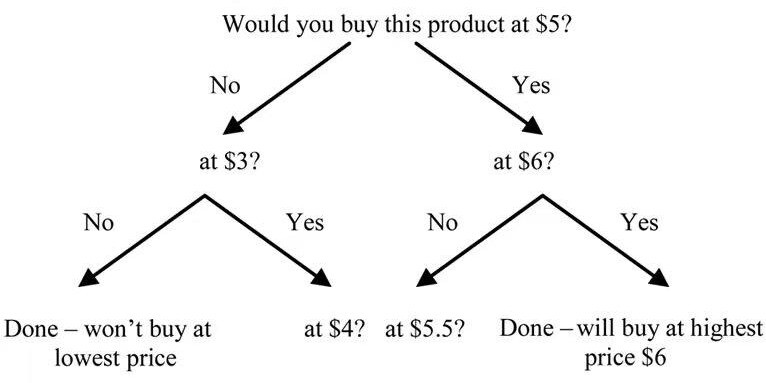
Figure 2. Gabor-Granger scheme of price eliciting.

A demand curve can be created by calculating the cumulative frequency distribution of the maximum prices respondents are prepared to spend on a specific product. An example with a real data from a marketing research project is presented in Figure 3.

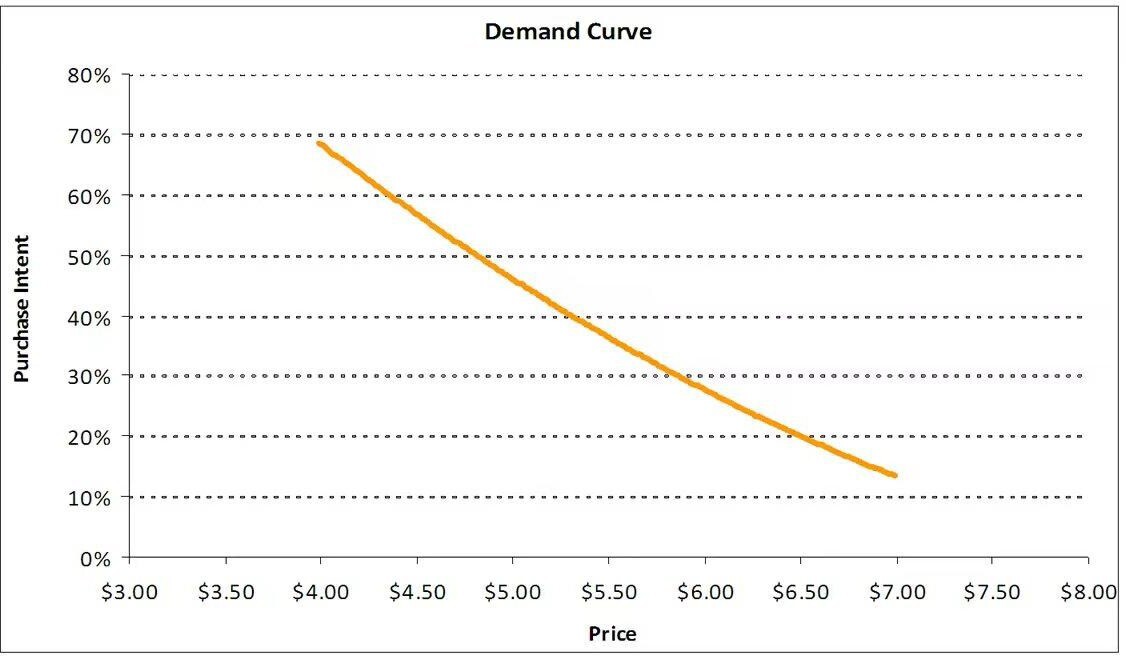
Figure 3. Gabor-Granger price model―the demand curve.

By multiplying each price point by its level of demand it is possible to consider the corresponding revenue curve―an example is given in Figure 4.

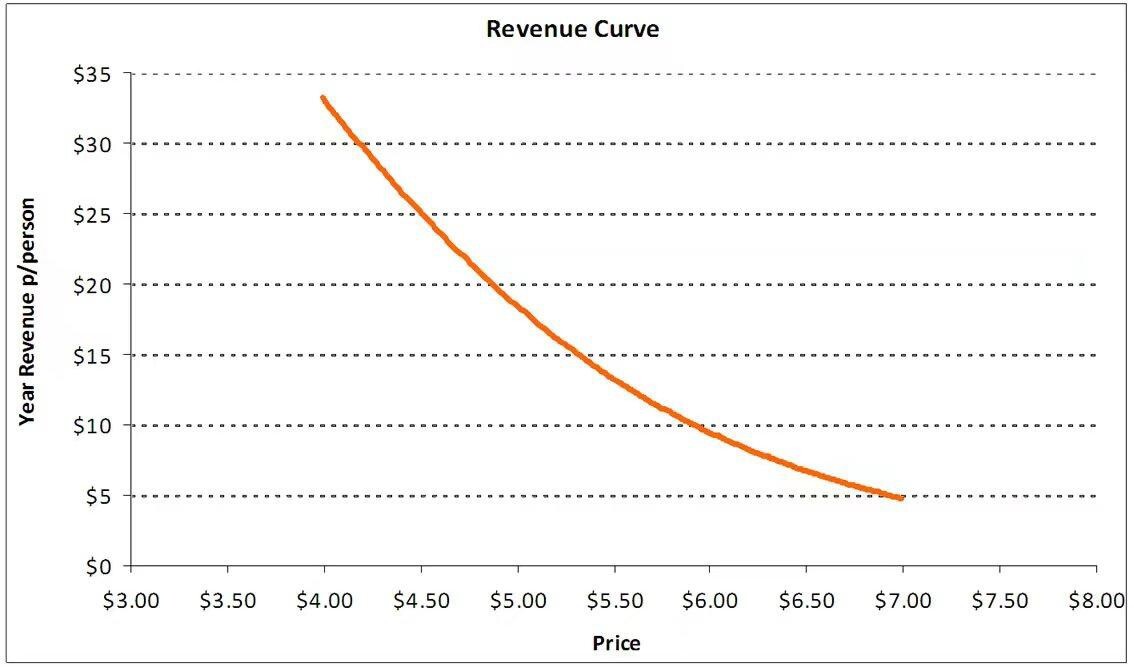
Figure 4. Gabor-Granger price model―the revenue curve.

The revenue curve can be utilized to identify an optimal price point that maximizes the projected revenue. Additional curve of a possible loss from optimal revenue is

presented in Figure 5.

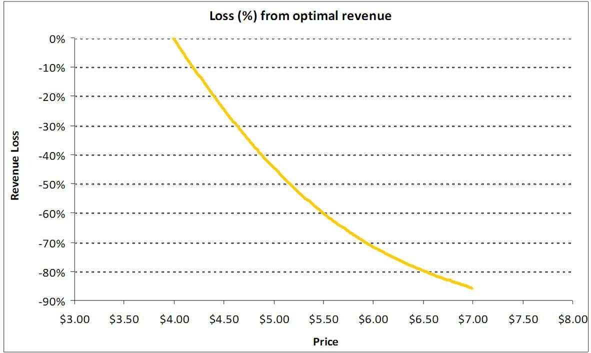
Figure 5. Gabor-Granger price model―the loss from optimal revenue curve.

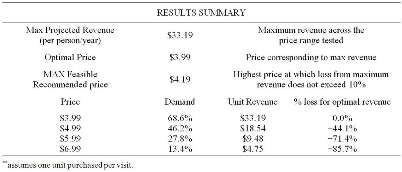
The results of GG-modeling can be summarized in the numerical Table 1 [6].

Table 1. The results of Gabor-Granger price modeling.

2.3 The importance of prisoner’s dilemma in pricing strategy

However, the limitations of these models are increasingly apparent: they can only give a rough range of the price of the product. Though possible payoffs of these prices can be drawn from a payoff matrix, it is still hard to determine which one is the maximum payoff the firm can get. Thus, in the pricing strategy, the focus is on the game itself. – often the process itself of developing the final price is as important as the price itself. And this process is frequently a game of prisoner’s dilemma in game theory.

In the previous studies, there are lots of good examples that using Game-Theory based dynamic pricing strategies in real life. And this model has many advantages as follows:

Indeed, game theory forms the basis for the design of electronic markets and is applicable in modeling the dynamic pricing problem in e-business markets. And, In recent times, game theory models have been employed in the domain of pricing network/internet resources. Within network environments, dynamic pricing can serve as an efficient approach to cost recovery, foster competition among diverse service providers, alleviate congestion, and regulate traffic levels [8].

The game theory framework is extensively utilized in the telecommunications sector for comprehending strategies among stakeholders and optimizing their payoffs. One of the most renowned illustrations is the wireless spectrum auction model that employs the game theory framework [5].

These findings suggest that the dynamic pricing model based on game theory is, in fact, a promising strategy for managing demand on the consumer side [15].

And, the prisoner's dilemma is a very classic and important example in game theory that greatly influences the study of Game-Theory based dynamic pricing strategies. In highly competitive markets, companies often engage in aggressive price wars to gain a larger market share. However, the prisoner's dilemma suggests that if both companies choose to lower prices, it may result in a destructive spiral where profits decline for both parties. Therefore, in pricing strategies, through game theory and the analysis of the prisoner's dilemma, we can see that if both companies adopt a cooperative strategy, it can create a stable market environment and achieve sustainable profitability. This is why many companies consider prisoner's dilemma when formulating pricing strategies.

In this project, the main goal is to demonstrate how and to what extent can prisoner’s dilemma in game theory be used in pricing strategies.

3 Discussion / Development

3.1 Transition from literature review to discussion

In the literature review, we have identified prisoner’s dilemma and basic strategies in prisoner’s dilemma according to Folk Theorem. Also, we have explored various studies and research papers related to pricing strategies. Now, in this discussion, we will build upon the existing literature on the prisoner's dilemma and examine the extent to which the prisoner's dilemma can be utilized in pricing decisions.

Our discussion will further explore the following aspects: The difference of pricing strategy in finite and infinite prisoner’s dilemma; the effects of strategies on potential payoffs under infinite prisoner’s dilemma; stability and sustainability of cooperative pricing agreements; how can Bayes’ theorem in prisoner's dilemma be applied to decision making of prices; limitations in using the prisoner's dilemma in pricing strategies.

By critically analyzing these aspects in discussion, we aim to contribute to the understanding of how the prisoner's dilemma and game theory can inform pricing strategies in practical finance settings.

3.2 Pricing strategy in infinite prisoner’s dilemma

3.2.1 Difference of pricing strategy in finite and infinite prisoner’s dilemma

In the literature review, we have already known that in finite prisoner’s dilemma, through backward induction, players will defect in every round by playing (D, D) which is the sub-game perfect Nash equilibrium. Therefore, the only pricing strategy in finitely repeated prisoner’s dilemma is that both firms choose the relatively lower prices, undercut each other's prices in each round in an effort to secure a larger share of the market.

However, in terms of infinite prisoner’s dilemma, due to the existence of an uncertain end, the situation is much more complex. Players are compelled to consider the long- term impact of their decisions. In this scenario, Grim Trigger strategy and the Tit- For-Tat strategy would become a more viable approach, since these two strategies can encourage players to adopt more moderate and predictable pricing behaviors, maintain stable and sustainable pricing, the mechanisms behind how these two strategies achieve this effect have been introduced in the literature review.

Next, we will investigate the effects of strategies taken by firms on their potential payoffs when pricing.

3.2.2 Pricing in Grim Trigger strategy

Before investigating the effect of Grim Trigger strategy and calculate its payoff when pricing, let us first introduce a concept called “discount factor”, also called “patient level” in game theory. It is a mathematical expression of how much someone values receiving a certain amount of money at a future date compared to receiving the same amount of money today. We use “δ” to represent it when calculation.

Let us give an example to explain “discount factor δ”, suppose that we leave a principal amount of 100 $ in an account for one year compounded annually, what is the future value of the account at the end of the year if the interest rate is r? The answer is 100·(1+ r). If we left it in for T years, then the future value of the account is 100·(1+ r)T. And we can flip the relation on its head to as the opposite question: for a given future cash flow occurring T periods from now, what is the present value of the cash flow worth today? To answer this, we just need to divide by the factor (1 + r). Or equivalently, multiply by the discount factor, 8 =1/(1+r).

In formal terms, the discount factor δ is a decimal number between 0 and 1 that is used to convert future cash flows into present value. The higher the discount factor, the greater the present value of future cash flows. Conversely, a lower discount factor means less weight placed on future cash flows and a greater emphasis on the current value of money.

Now let us get back to the topic.

Suppose, in the case of pricing strategy, two firms1 and 2 are interacting repeatedly for the payoff of different possible prices and the short-term payoff are drawn by the prisoner’s dilemma (see figure 6). We use C to denote “cooperation” strategy which means the firm sets a relatively higher price, and we use D to denote “Defect” strategy which means the firm sets a relatively lower price.

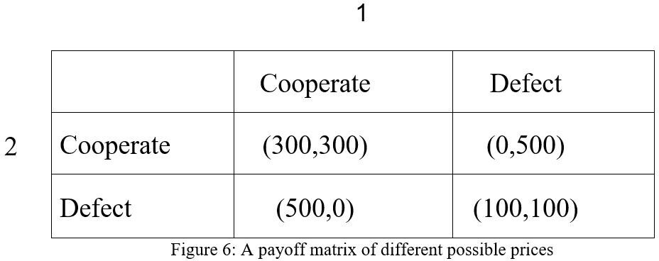
Figure 6. A payoff matrix of different possible prices

Suppose that both firms adopt the grim trigger strategy, and they play (C, C) at the beginning of the game. Then there are two situations, one is no-deviation: For the rest of the game, they will continue play (C, C) if nobody plays D. The other situation is deviation: If one or two firms ever play D, then both firms will play (D, D) forever according to the grim punishment.

Next, we will calculate the payoff of firm 1(or firm 2, since the game is symmetric) to analyze which situation results in a higher payoff. Additionally, we will determine the conditions in which the firm would prefer to adopt this situation.

In the first situation, no-deviation stream of payoffs for firm1 is (300, 300, . . .), whose discounted average is 300. Now let us compute the net present value of cooperating forever, which equals to 300+300δ+300δ²+…. Simplify the equation, we get 300(1+δ+δ²+…) which is a convergent geometric series(1+δ+δ²+δ³+δ4+δ5

+…=1/1-δ). Thus, the payoff equals to 300/1-δ.

In terms of the situation that defects, firm2 adopts a strategy that generates a different sequence of outcomes, which means there is at least one period in which it chooses D. In all subsequent periods player 1 chooses D according to the grim punishment, so the best deviation for player 2 chooses D in every subsequent period, since D is her unique best response to D. we draw a diagram to show the payoff from defecting:

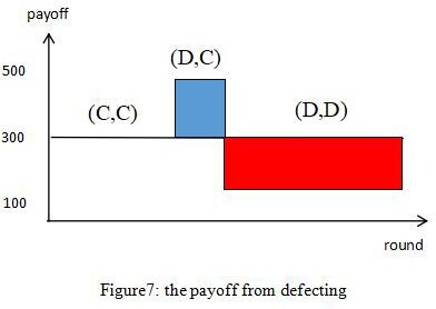
Figure 7. The payoff from defecting

The blue area represent immediate gain from defecting, and the red area represent future loss from defecting in the punishment phase. While it looks like an easy task in the diagram (since the red area seems to outweigh the blue area), we need to remember that people have a preference for receiving things sooner rather than later - this preference will magnify the size of the blue area and shrink the size of the red area, psychologically.

Therefore, the net present value of the payoff stream when a player defects and is then punished for the rest of the game, we can build the equation according to it :500+100δ+100δ²+…. Simplify the equation, it’s equal to 500+100δ(1+δ+δ²+…), using the same convergent geometric series result, we can find that: 500+ 100δ/1-δ.

We now compare payoffs of the firm from cooperating and defecting when pricing, if its present value calculation of cooperation payoff stream is greater than deviation payoff, then they will cooperate. We can establish an inequality to express it:

300/1-δ ≥ 500+ 100δ/1-δ.

300≥500-500δ+100δ

δ ≥ 1/2

This indicates that both firms will choose to cooperate when pricing, if the firm's concern for future earnings is greater than or equal to half of their concern for current earnings.

In this part, we analyze in detail the effect of grim trigger strategies on potential payoffs of firms when pricing, including cooperative pricing, non-cooperative pricing. We suggest that while non-cooperative pricing strategies may lead to short-term gains, they often result in a loss for both parties in the long run. Cooperative pricing agreements, on the other hand, promote mutual benefits and long-term stability (Figure 7). We then compared the payoffs under different pricing strategies, and found that it was related to the patience level of the firm itself.

3.2.3 Pricing in Tit-For-Tat strategy

Now consider the firms use the tit-for-tat strategy when pricing. There are also two situations, one is no-deviation, the other is deviation. However, the defecting situation is more complex than in Grim Trigger strategy.

Suppose that at the beginning of the game, firm1 plays C. Then, if firm 2 also choose to cooperate, then the payoff in each round is 300. We can now calculate the present value of perpetual cooperation, which is equivalent to 300+300δ+300δ²+…. Simplifying the equation yields 300(1+δ+δ²+…), which is a convergent geometric series. Therefore, the payoff amounts to 300/1-δ. The payoff is exactly the same as in Grim Trigger strategy.

However, for the defecting payoff, firm1 has two options. Suppose that both firms play (C, C) at the first period of the game. Then, as above, if player 1 can gain by defecting then it can gain by choosing D in the second period. If it does so, then firm 2 will choose D in the third period in order to punish it, and continues to choose D until firm 1 returns to C. Thus firm 1 has two options: it can return to C, in which case in the next period it faces the same situation as she did at the start of the game, or she can continue to choose D, in which case player 2 will continue to do so too, which means both firms take turns cooperating and defecting. We draw a table to indicate the game:

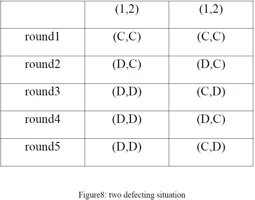
Figure 8. Two defecting situation

We conclude that if firm 1 can increase its payoff by defecting then it can do so either by choosing D in every period or by alternating between D and C.

In the first defecting situation, through the table, we find the payoff is 500+100δ+100δ²+…. Simplify the equation, it’s equal to 500+100δ(1+δ+δ²+…), using the same convergent geometric series result, we can find that: 500+ 100δ/1-δ.

In terms of second defecting situation, the equation is 500+ 0·δ+500·δ²+0·δ³+…, simplify, we get 500(1+δ²+δ⁴+δ⁶+…). This time, the equation is not a convergent geometric series. We need to find a way, using geometric series represent this equation. The following is the mathematical derivation process:

We know that geometric series:1+δ+δ²+δ³+δ4+δ5 +…=1/1-δ. This formula can also be expressed as: (1+δ²+δ⁴+δ⁶+…)+(δ+δ³+δ⁵+…)=1/1-δ. And the term (δ+δ³+δ⁵+…) can be expressed as: δ(1+δ ² +δ4+δ6+ … ).Then,(1+δ ² +δ4+δ6+ … ) +δ · (1+δ ²

+δ⁴+δ⁶+…)=1/1-δ. We finally get (1+δ²+δ⁴+δ⁶+…)=1/(1-δ)(1+δ).

Therefore, 500(1+δ²+δ4+δ6+…) in the second defecting situation equals to 500/(1- δ)(1+δ).

We compare payoffs of the firm from cooperating and defecting when pricing, we need to establish two inequalities to express it:

300/1-δ ≥500+ 100δ/1-δ And 300/1-δ ≥500/(1-δ)(1+δ). δ ≥ 1/2 and δ ≥ 2/3

This means that in first defecting situation, two firms will choose to cooperate only if their patient level is greater than or equal to 1/2. In second defecting situation, they need to be more patient than in situation one if they cooperate, since their patient level is greater than or equal to 2/3.

In this part, we analyze in detail the impact of tit-for-tat strategies on potential payoffs of firms when pricing, including one cooperative pricing and two non- cooperative pricing, we also analyse the difference of two non-cooperative pricing. Then, we compared the payoffs under different pricing strategies, and found that it was related to the patience level of the firm itself.

3.2.4 Stability and sustainability of cooperative pricing strategy

In the prisoner's dilemma, cooperation is a rational choice that maximizes the benefits for both parties involved. However, due to the potential for defecting, the stability and sustainability of cooperative pricing agreements face challenges. In this part, we will investigate the stability and sustainability of cooperative pricing agreements, and under what circumstances would their cooperation breakdown. We have drawn three graphs to represent three situations respectively:

First situation, both firms’ δ is actually higher than 1/2, that means they think the present value from cooperating in that payoff stream is greater than the present value they get from defecting. Thus, in this particular case, they will choose to cooperate, and the cooperative pricing agreement is suitable. (Figure9)

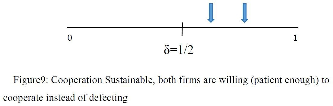
Figure 9. Cooperation Sustainable, both firms are willing (patient enough) to cooperate instead of defecting

In the second situation, firm2 is willing to cooperate, because it thinks the present value from cooperating in that payoff stream is greater than the present value they get from defecting. However, firm1 is very impatient, since it’s δ is close to 0. His present value calculation of payoff stream of cooperation is not as big as present value of defecting. Thus, it will choose to defect. The cooperative pricing agreement is not sustainable. (Figure10)

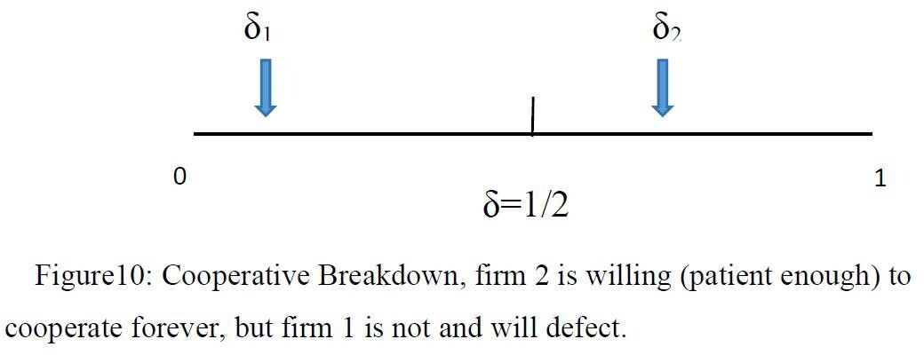
Figure 10. Cooperative Breakdown, firm 2 is willing (patient enough) to cooperate forever, but firm 1 is not and will defect.

In the last case, both firms have the value of δ less than 1/2, unfortunately, neither of them is willing to cooperate. The cooperative pricing agreement is breaking down, since they are both very impatient. (Figure11)

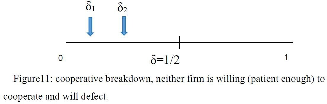
Figure 11. Cooperative breakdown, neither firm is willing (patient enough) to cooperate and will defect.

In this part, we have drawn three diagrams respectively to analyse in which situation the cooperative pricing agreements will breakdown, this is related to their patient level. Based on the above three situations, in pricing strategy, we can judge whether the other firm will choose high price or low price by predicting its level of patience. According to this, we can decide and adjust our final price to maximum our payoff.

3.3 Develop a probabilistic model based on Bayes’ theorem in the prisoner’s dilemma

In the previous discussion, we have investigated the impact of basic strategies in the infinite prisoner's dilemma on potential payoffs when pricing. Their characteristic is that both firms having a clear understanding of each other's strategy set and payoff situation, which is known as a game with perfect information.

However, in real-life situations, there are many cases where game participants do not have complete knowledge of each other's strategy set and payoff situation, leading to an incomplete perfect information game. A typical example of an incomplete perfect information game is the study of market pricing strategies. In market competition, companies often lack accurate information about each other's costs, demand curves, and market responses. Therefore, when setting prices, companies face uncertainty and cannot determine what strategy the other party will choose, whether it be cooperation or deviation. This uncertainty presents even more complex challenges for game analysis.

Next, we are going to develop a probabilistic model based on the Bayes’ theorem to address the uncertainty in pricing problems, aiming to accurately predict the opponent's behavior and maximize one's own interests.

Before we begin our discussion, let us give a brief introduction to Bayes’ formula, which is a method for updating probability estimates.

P(A|B) = (P(B|A)·P(A)) / P(B)

In this formula, the conditional probability P(A|B) represents the probability of event A occurring given that event B has occurred, while the prior probabilities P(A) and P(B) represent the probabilities of events A and B occurring on their own.

To summarize the role of the Bayesian formula in a simple and informal way: when additional information about the subject of study becomes available, the Bayesian formula can be used to revise the prior probabilities and obtain more accurate

posterior probabilities.

Now, we begin to develop the probabilistic model. We first need to collect empirical data and list potential payoffs of the possible prices. Then, based on the behavior and outcomes of both firms in multiple game rounds, I will calculate the probability of the opponent choosing cooperation or deviation. I will update these probabilities using Bayesian formula and ultimately deduce whether the company should choose cooperation or deviation.

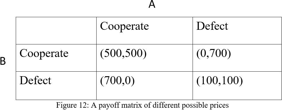
Figure 12. A payoff matrix of different possible prices

Suppose in this case (see figure 12). There are two assumptions of A, one is the cost of A choose to defect is high, the other is the cost of A choose to defect is low. A will choose to cooperate and defect respectively in this two situations.

Before the first round of the game, suppose that B’s prior assumptions of A’s type and behavior is as follow:

If the P(the cost of A choose to defect is high)=0.7, then the P(A chooses to cooperate)=1. However, if the P(the cost of A choose to defect is low)=0.3, then the P(A chooses to cooperate)=0.2.

According to this prior assumptions of A, we can calculate that the probability of A choosing to cooperate which is considered as prior probability is 0.7·1+0.3·0.2=0.76.

After the first round of the game, A chooses to cooperate. Now we can use the Bayes' theorem to update the probabilities based on new information. P(high cost of defecting | cooperate) = (P(cooperate | high cost of defecting) · P(high cost of defecting)) / P(cooperate)=0.7·1/0.76=0.92

Now, the probability that B thought A being high cost will change from 0.76 to 0.92(updated). The probability situation at this time is as follow:

If the P(the cost of A choose to defect is high)=0.92, then the P(A chooses to cooperate)=1. However, if the P(the cost of A choose to defect is low)=0.08, then the P(A chooses to cooperate)=0.2.

Now we are entering the second round of the game, and A still choose to cooperate with B. Therefore, P(A choose to cooperate)=0.92·1+0.08·0.2=0.936

Correspondingly, the probability that B thought A being high cost will update again, use the Bayes’ theorem, we get P(high cost of defecting | cooperate) = (P(cooperate | high cost of defecting) · P(high cost of defecting)) / P(cooperate)=0.92·1/0.936=0.983

In the two consecutive rounds of the game, B's belief about the probability of A belonging to the high-cost category changed from 0.7 to 0.92 and then to 0.983. Therefore, it can be deduced that A is a high-cost type of firm when defecting, which means it will choose to cooperate when pricing instead of defecting. Therefore, rational B should choose to defect, the optimal pricing strategy for firm B is relatively lower price, since it can maximum its payoff.

In summary, we develop a probabilistic model based on Bayes’ theorem, it can provide us with another decision-making pattern for our pricing strategy. Compared to pricing strategies in prisoner's dilemma, Bayes’ game-based strategies have some advantages. First, Bayes’ theorem allow for the incorporation of uncertainty and incomplete information into the pricing decision-making process. This enables businesses to adapt their pricing strategies based on changing market conditions and competitor behavior. Second, Bayes’ theorem models provide a framework for dynamic pricing strategies. Businesses can continuously update their pricing decisions based on new information and feedback from the market, allowing for more agile and adaptive pricing approaches.

3.4 Limitation of prisoner’s dilemma in pricing

In this project, we have already investigated the effects of prisoner’s dilemma when pricing, using two basic strategies and Bayes’ theorem. However, there are some limitations when using these methods in real-life situations.

When we investigate the effects of two basic strategies on their potential payoffs in

pricing.

One limitation point is that in both strategies, each side will correspond to the other's previous actions. If one company lowers its prices, the other will also lower its prices. This can lead to a price war, where the two companies continually lower prices to gain a competitive advantage. Such a situation could harm profitability and create an unstable market environment.

In this regard, we suggest adopting a relatively mild strategy. For example, when the opponent chose to defect in the last round, it will choose to defect with probability p in this round. This can not only alert the opponent not to defect, but also effectively avoid the problem that cooperation cannot be achieved again due to deviation caused by unexpected factors.

When Bayesian theorem applied to prisoner's dilemma in pricing, some people believe that it also has some limitations.

One limitation is the assumption of perfect information and prior probability. Bayesian theorem requires that all parties have complete and accurate information about the market and their competitors. In reality, this is not always the case, and firms may have incomplete or inaccurate information set. This can lead to incorrect assumptions and decisions based on the Bayesian calculations.

In this regard, we need to clarify that Bayesian theorem does not require both firms to have complete and accurate information when pricing. On the contrary, it is a method for modeling uncertainty and making inferences and predictions in situations of incomplete information. By observing market feedback and the actions of competitors, firms can continuously adjust their information set and probability distribution to optimize their pricing strategies.

4 Conclusion

The purpose of the current study was to determine the extent of prisoner's dilemma used in pricing strategies, and how the prisoner's dilemma is used in pricing strategies. This dissertation explores the following aspects: the effects of strategies taken by firms on their potential payoffs when pricing; stability and sustainability of cooperative pricing agreements; how can Bayes’ theorem in prisoner's dilemma be applied to decision making of prices.

In terms of research methods, we first sorted out and summarized the prisoner's dilemma theory and common pricing strategies, then introduced the importance of game theory based pricing strategies in the literature review section. In the discussion section, we discussed the impact of different strategies adopted by companies on their potential payoffs, this study has shown that the company's own patience level plays an significant role in pricing, we also suggest that while non-cooperative pricing strategies may lead to short-term gains, they often result in a loss for both parties in the long run. Cooperative pricing agreements, on the other hand, promote mutual benefits and long-term stability. Then we studied the stability and sustainability of the cooperative pricing agreement, and found that we can predict the other firm's choices based on its level of patience, and adjust our own choices accordingly to maximize benefits. Finally, in a more realistic scenario, a pricing strategy model is developed using Bayesian theorem in prisoner’s dilemma.

Our research has important implications for economics, marketing and game theory. First, by applying prisoner's dilemma theory, companies can better understand the competitive environment and develop more effective pricing strategies. Secondly, the research results can provide reference for enterprises to help them make wise decisions when facing competition, thereby improving market efficiency and profits. In game theory, the Bayesian formula is also found to be applied to the prisoner's dilemma.

However, our study still has some limitations. First, our research is limited to the application of prisoner's dilemma theory in pricing strategies, and the impact of other factors has not been fully considered. Secondly, according to the prisoner's dilemma pricing strategy, if one firm defects, it may lead to a price war and create an unstable market environment. Finally, in the study of Bayesian games, the prior probability may be imprecise, causing the model to be unable to accurately predict the opponent's decision-making.

In the future research, considerably more work will need to be done to determine the impact of other factors on pricing and solve the problem of defecting due to unexpected factors and the inability to cooperate again. It is also necessary to use

deep learning models and artificial intelligence to collect historical data and market information, in order to more accurately predict the prior probability of opponents.

In conclusion, the prisoner's dilemma plays a significant role in pricing strategies adopted by businesses, but it also has certain limitations when used. We believe that through in-depth research on the application of the prisoner's dilemma, more comprehensive and scientific pricing strategies can be developed to ensure sustainable market development.

References

[1]. Dolgui, A., & Proth, J. M. (2010). Pricing strategies and models. Annual Reviews in Control, 34(1). https://doi.org/10.1016/j.arcontrol.2010.02.005
[2]. Friedman, J. (1971). A non-cooperative equilibrium for supergames. Review of Economic Studies, 38(1), 1–12. https://doi.org/10.2307/2296617
[3]. Dean, J. (1976). Pricing policies for new products. Harvard Business Review, 54(6), 141–153.
[4]. Kuhn, S. (2019). Prisoner’s dilemma. Stanford Encyclopedia of Philosophy. https://plato.stanford.edu/entries/prisoner-dilemma/
[5]. Kumar, R., Crawford, S., & Stewart, D. (2023). Pricing models for 5G multi-tenancy using game theory framework. IEEE Communications Magazine, 1–2. https://doi.org/10.1109/mcom.001.2200742
[6]. Lipovetsky, S., Magnan, S., & Zanetti-Polzi, L. (2011). Pricing models in marketing research. Intelligent Information Management, 3(5), 2–4. https://doi.org/10.4236/iim.2011.35020
[7]. Salish, M. S. (2020). Prisoner’s dilemma. INOMICS. https://inomics.com/
[8]. Narahari, Y., Ramasuri, N., & Prakash, N. (2005). Dynamic pricing models for electronic business. Sadhana, 30(2–3), 240–241. https://doi.org/10.1007/bf02706246
[9]. Osborne, M. J., & Rubinstein, A. (2001). A course in game theory. Cambridge, MA: MIT Press.
[10]. Osborne, M. J. (2003). A course in game theory. MIT Press.
[11]. Osborne, M. J., & Rubinstein, A. (2001). Infinitely repeated games vs. finitely repeated games. In A course in game theory (pp. 134–136). Cambridge; London: MIT Press.
[12]. Pettit, P., & Sugden, R. (1989). The backward induction paradox. The Journal of Philosophy, 86(4). https://doi.org/10.2307/2026960
[13]. Sammut-Bonnici, T., & Channon, D. (2015). Pricing strategy. In Wiley Encyclopedia of Management (pp. 1–2). https://doi.org/10.1002/9781118785317.weom120162
[14]. Sigmund, K. (2010). The calculus of selfishness. Princeton: Princeton University Press.
[15]. Srinivasan, D., Pandey, M. N., & Cheong, S. H. (2017). Game-theory based dynamic pricing strategies for demand side management in smart grids. Energy, 126, 142–143. https://doi.org/10.1016/j.energy.2016.11.142
Cite this article
Wang,Z. (2024). To what extent can prisoner’s dilemma in game theory be used in pricing strategy?. Advances in Operation Research and Production Management,3,1-13.
Data availability
The datasets used and/or analyzed during the current study will be available from the authors upon reasonable request.
Disclaimer/Publisher's Note
The statements, opinions and data contained in all publications are solely those of the individual author(s) and contributor(s) and not of EWA Publishing and/or the editor(s). EWA Publishing and/or the editor(s) disclaim responsibility for any injury to people or property resulting from any ideas, methods, instructions or products referred to in the content.
About volume
Journal:Advances in Operation Research and Production Management
© 2024 by the author(s). Licensee EWA Publishing, Oxford, UK. This article is an open access article distributed under the terms and
conditions of the Creative Commons Attribution (CC BY) license. Authors who
publish this series agree to the following terms:
1. Authors retain copyright and grant the series right of first publication with the work simultaneously licensed under a Creative Commons
Attribution License that allows others to share the work with an acknowledgment of the work's authorship and initial publication in this
series.
2. Authors are able to enter into separate, additional contractual arrangements for the non-exclusive distribution of the series's published
version of the work (e.g., post it to an institutional repository or publish it in a book), with an acknowledgment of its initial
publication in this series.
3. Authors are permitted and encouraged to post their work online (e.g., in institutional repositories or on their website) prior to and
during the submission process, as it can lead to productive exchanges, as well as earlier and greater citation of published work (See
Open access policy for details).