1. Introduction

As one of the most important aspects of a country’s overall economic performance, Gross Domestic Product (GDP) represents the total value of all goods a services produced in a given area over a given period. GDP is a key component in measuring a country’s overall economic growth, assessing the actions of policy decisions, and determining economic development strategies. Given the significance of GDP, the accurate forecasting of GDP has become one of the most important aspects of a macroeconomic forecast. An accurate GDP forecast is essential in analyzing future trends for makers, investors, and government policy, as it plays a role in allocation of resources, forecasting, and planning.

In recent decades, a variety of statistical and econometric methods have emerged to model and predict GDP. One of the methods used was the Autoregressive Integrated Moving Average (ARIMA) model, proposed by Box and Jenkins, which has emerged as quite popular due to its ease of use and performance in forecasting (in the univariate context) [1]. A substantial body of empirical research has also been conducted, demonstrating that ARIMA models are effective for forecasting GDP. These studies have been conducted for Egypt [2], Kenya [3], India [4], Bangladesh [5], and the African continent [6].

In addition to GDP, ARIMA models have also been successfully applied to forecast various economic and financial variables such as CPI [7], commodity prices [8], and stock prices [9,10]. Some studies have gone further to compare ARIMA with more advanced machine learning models like LSTM, highlighting both the strengths and limitations of ARIMA in complex forecasting tasks [11,12].

This paper proposes to find the best ARIMA model to forecast China’s GDP from 2025 to 2029 using annual GDP data from 1960 to 2024. We will take the Box-Jenkins approach to examine a range of ARIMA models and compare them to find the most suitable model for our data.

2. Literature review

2.1. Empirical studies on GDP forecasting using ARIMA

Numerous studies have applied ARIMA models to forecast national GDP, demonstrating their effectiveness across different economic settings. For example, Abonazel and Abd-Elftah [2] used an ARIMA(1,2,1) model to predict Egypt’s GDP from 1965 to 2016, selecting the best model based on AIC and residual diagnostics. Mungai [3] studied Kenya’s GDP from 1960 to 2012 using the Box-Jenkins approach and selected ARIMA(2, 2, 2) as the best-fitting model based on AIC and stationarity tests. The model showed good predictive accuracy, with in-sample forecasts deviating less than 5%, and was used to forecast GDP for the next five years. In the case of Bangladesh, Bhuiyan et al. [5] modeled Bangladesh’s manufacturing GDP and confirmed that ARIMA models can effectively capture economic patterns. Despite these contributions, ARIMA-based studies focusing on China remain limited. Ning et al. [13] analyzed a regional GDP series for Shaanxi province using a shorter time frame. In contrast, this study has a longer national series from 1960 to 2024 and forecasts China’s GDP through 2029, thus providing a more comprehensive perspective.

2.2. ARIMA versus alternative forecasting methods

Although ARIMA models are commonly used for forecasting in economics due to their interpretability and good theoretical foundation, they have limitations due to the nature of economic data, which can exhibit complex nonlinear correlations. More modern machine learning models, such as Long Short-Term Memory (LSTM) neural networks, on the other hand, performed well at reflecting the historical nonlinear dependencies within time series data.

Siami-Namini and Namin [11] conducted a number of large-scale empirical comparisons of LSTM and ARIMA models over multiple economic and financial datasets and found consistently better accuracy performance from LSTM models than ARIMA models. Similarly, Sirisha et al. [12] concluded that LSTM models produced superior performance compared to ARIMA and SARIMA models in forecasting profit levels.

Nonetheless, deep learning models such as LSTM models typically require significantly more training data, have higher computational costs, and provide less interpretability than a traditional statistical model. Thus, in small-sample, single-variable economies such as GDP models, ARIMA provides a more practical and interpretable solution.

2.3. Autoregressive Integrated Moving Average (ARIMA) models

2.3.1. Moving-average (MA) model

The moving-average (MA) model is one of the fundamental components in time series analysis. It represents the current value of a time series as a linear combination of current and past white noise error terms. Specifically, a time series  $$ \left\{x_t\right\}$$  is said to follow an MA(q) process if it can be written as:

$$ \begin{array}{c}{X}_t={\epsilon }_t-{\theta }_1{\epsilon }_{t-1}-{\theta }_2{\epsilon }_{t-2}-\cdots -{\theta }_q{\epsilon }_{t-q}\end{array}$$(1)

where εt denotes a white noise error term at time t, and θ1 ,θ2,...,θq are the model parameters. This model captures short-term dependencies in the data by expressing  $$ x_t$$  in terms of a finite number of past forecast errors. Since only a limited number of lags are involved, the MA model is typically classified as a short-memory process [1].

2.3.2. Autoregressive (AR) model

The autoregressive (AR) model describes a time series where the current value depends linearly on its previous values. An AR(p) process of order p is defined as:

$$ \begin{array}{c}{X}_t={\varphi }_0+{\varphi }_1{X}_{t-1}+{\varphi }_2{X}_{t-2}+\cdots +{\varphi }_p{X}_{t-p}+{\epsilon }_t\end{array}$$(2)

where  $$ x_t$$ is the value of the time series at time t, ϕ0 is a constant term,  $$ \mathrm{\varphi }1,\mathrm{\varphi }2,...,\mathrm{\varphi }\mathrm{p}$$  are the autoregressive coefficients, and εt is a white noise error term with zero mean and constant variance.

Unlike the MA model, the AR model allows past values of the series to influence the current observation, often resulting in longer memory and persistence in the data. The autocorrelation function (ACF) of an AR process typically decays gradually, which is a key indicator in identifying its structure [1].

2.3.3. Autoregressive Moving Average (ARMA) model

The ARMA model combines the properties of both the autoregressive (AR) and moving average (MA) models. A time series  $$ {\{x}_t\}$$  is said to follow an ARMA(p, q) process when it incorporates both p lagged values of the series and q lagged error terms. The general form of the model is:

$$ \begin{array}{c}{X}_t={\varphi }_0+{\varphi }_1{X}_{t-1}+\cdots +{\varphi }_p{X}_{t-p}+{\epsilon }_t-{\theta }_1{\epsilon }_{t-1}-\cdots -{\theta }_q{\epsilon }_{t-q}\end{array}$$(3)

In this structure, ϕi represents the autoregressive parameters and  $$ {\theta }_j$$ denotes the moving average coefficients. The error term εt is assumed to be white noise. By incorporating both past values and past errors, the ARMA model is capable of capturing more complex time series dynamics compared to the AR or MA models individually [1].

2.3.4. Autoregressive Integrated Moving Average (ARIMA) model

The ARIMA model generalizes the ARMA framework to accommodate non- stationary time series by introducing a differencing component. In an ARIMA(p,d,q) model, p denotes the order of the autoregressive part, d represents the number of times the series is differenced to achieve stationarity, and q is the order of the moving average part.

When a time series { $$ x_t$$ } exhibits non-stationary behavior, differencing is applied d times to obtain a stationary series  $$ \{\nabla \mathrm{d}{x}_t\}$$ . A first-order differenced ARIMA(p,1,q) model can be written as:

$$ \begin{array}{c}\nabla X_t={\varphi }_0+{\varphi }_1\nabla X_{t-1}+\cdots +{\varphi }_p\nabla X_{t-p}+{\epsilon }_t-{\theta }_1{\epsilon }_{t-1}-\cdots -{\theta }_q{\epsilon }_{t-q}\end{array}$$(4)

where  $$ \nabla x_t\mathrm{ }=\mathrm{ }{x}_t\mathrm{ }-\mathrm{ }{x}_{t-1}$$  represents the first difference of the original series. If both p and q are set to zero, the model reduces to a simple random walk, which corresponds to an ARIMA(0,1,0) process. This extension makes ARIMA models particularly suitable for real-world economic and financial data, which often exhibit trends or evolving variance over time [1].

2.4. Box-Jenkins methodology

The Box–Jenkins approach, introduced by George Box and Gwilym Jenkins in the early 1970s, is a systematic approach for identifying, estimating, and checking ARIMA models in time series modelling. The Box–Jenkins procedure is intended to provide the best statistical fit of a model to past observations of a univariate time series. The Box–Jenkins procedure iterates on diagnostics and modifications to ensure that the model captures the basic data structure with minimal residual autocorrelation [1]. The Box–Jenkins process involves four steps, as shown in Figure 1.

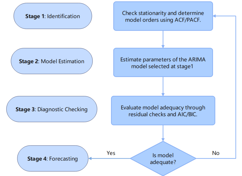
In Stage 1, we will assess the stationarity of the time series via a series of tests and differencing non-stationary data until stationarity is achieved. The plots of the autocorrelation function (ACF) and partial auto- correlation function (PACF) will be examined to suggest appropriate orders for the autoregressive (p) and moving-average (q) components of our model. The outcome of this step will provide an initial candidate ARIMA(p, d, q) model for validation.

After selecting the model, the parameters of our model will be estimated using either maximum likelihood estimation (MLE) or non- linear least squares methods, which seek to provide the best model by optimally estimating the relationship between the actual and predicted values while ensuring that these estimates are statistically consistent.

Then in Stage 3, the adequacy of the fitted model is evaluated. We want to ensure the residuals are representative of white noise (i.e., they should be uncorrelated, normally distributed, and homoscedastic). We will use diagnostic tests like the Ljung–Box test, and ACF/PACF plots ofthe residuals. We will also compare the model performance using information criteria like the Akaike Information Criterion (AIC) and Bayesian Information Criterion (BIC), defined as follows:

$$ \begin{array}{c}\mathrm{A}\mathrm{I}\mathrm{C}=2m-2\ln (\widehat{L}),\hspace{1em}\mathrm{B}\mathrm{I}\mathrm{C}=\ln (n)m-2\ln (\widehat{L})\end{array}$$(5)

where denotes the maximum value of the likelihood function, m is the number of estimated parameters, and n is the sample size. Lower values of AIC or BIC indicate a more optimal balance between model complexity and goodness of fit.

Once a model passes the diagnostic checks, it can be used to produce forecasts. A validated ARIMA model provides reliable short-term projections by effectively modeling the underlying dynamics of the time series in a statistically sound manner.

3. ARIMA model estimation and GDP forecasting

3.1. Data description

This analysis uses annual GDP data for China from the World Bank over the period 1960-2024, which consists of 65 observations. This is well above the generally accepted minimum of 50 observations for ARIMA data in the Box–Jenkins paradigm, and the measurements are in current US dollars (USD).

3.2. Stationarity and preliminary analysis

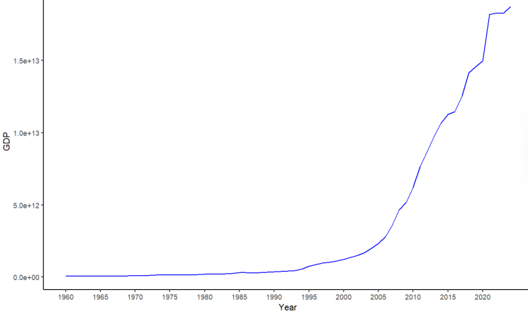
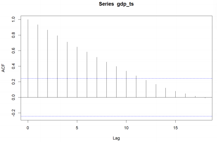
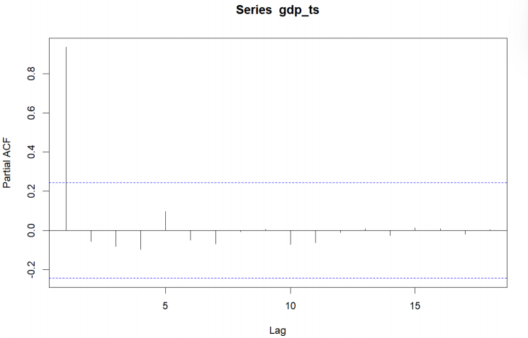
A simple, direct look at the original GDP series (Figure 2) shows a clear exponential upward trend over time (particularly after the early 2000s), which leads to the assumption that there may be non-stationarity in the series, which would violate the assumptions necessary for ARIMA processes. To determine whether the data were non-stationary, the autocorrelation function (ACF) and partial autocorrelation function (PACF) were reviewed (Figure 3 and Figure 4). The ACF shows evidence of slowly decaying while the PACF noticeably spikes at lag 1 and drops off quickly, which indicates the existence of non-stationarity.

The Augmented Dickey–Fuller (ADF) test was used to verify this statistically. The ADF test returned a p-value of 0.978, which is much larger than the common threshold of 0.05, meaning that the unit root null hypothesis can not be rejected. Thus, the series is nonstationary.

To create a stationary series, we logarithmically transformed the original series and performed first-order differencing. The resulting series is much less volatile, as demonstrated in Figure 5, but it still shows some signs of non-stationarity. The ADF test gives a p-value of approximately 0.167, indicating that the series is still non-stationary at the 5% significance level.

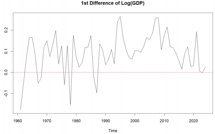
Therefore, additional differencing is required before fitting an ARIMA model.

Then, a second-order difference to the natural logarithm of the GDP series was applied. As shown in Figure 6, the series becomes more stable and fluctuates around a constant mean (0). The ADF test returns a p-value of 0.01, confirming stationarity at the 5% level. Based on this, we determine that the differencing order is d=2.

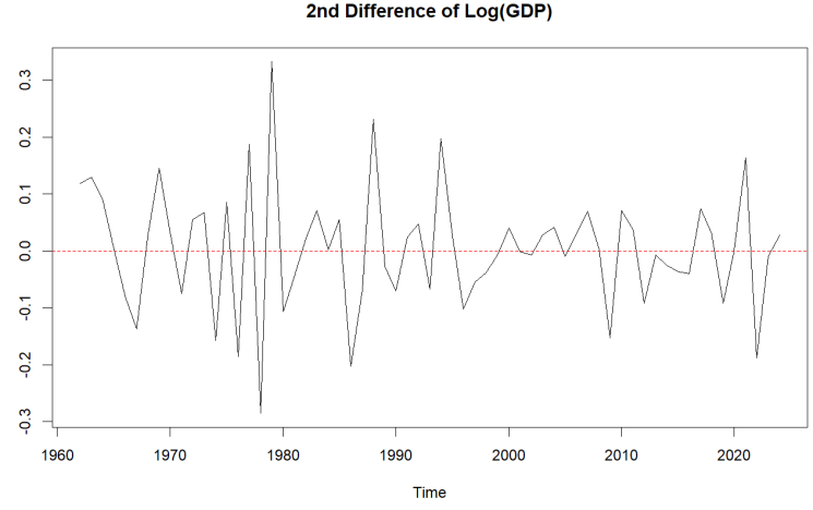
The transformation is defined as:

$$ \begin{array}{c}{X}_t=\ln (GD{P}_t)-\ln (GD{P}_{t-2})\end{array}$$(6)

where ln(GDPt ) denotes the natural logarithm of the GDP at time t.

3.3. Model identification and selection

After performing second-order differencing on the log-transformed GDP series, we examined the Autocorrelation Function (ACF) and Partial Autocorrelation Function (PACF) plots with a view to determining the appropriate ARIMA model structure.

In the ACF plot (Figure 7), we observe a significant negative spike at lag 1 with a rapid decay. The PACF plot (Figure 8) shows a significant value at lag 1, then diminishes rapidly at subsequent lags. This pattern suggests the data has both an order one autoregressive (AR) and a moving average (MA) component.

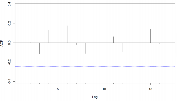
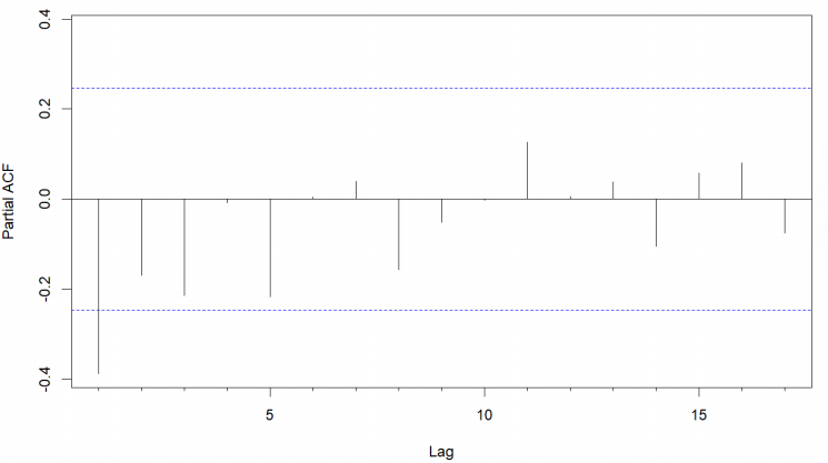
Based on the analysis, the ARIMA(1,2,1) model seems to be an acceptable choice for modeling the transformed GDP. This model will be further validated during the parameter estimation and diagnostic checking stages.

The results of the estimation of the ARIMA(1,2,1) model are presented in Table 1. The AR(1) coefficient is not statistically significant at the level 5% (p=0.1364), which indicates a weak autoregressive effect. In contrast, the MA(1) coefficient is highly significant (p<0.001), suggesting a strong moving average component in the model. Despite the insignificance of AR(1), the overall model is still considered reasonable, as the residuals show minimal autocorrelation and the model achieves low forecast errors. Therefore, the ARIMA(1,2,1) model can be deemed a suitable choice for capturing the dynamics of the GDP time series.

To determine the optimal ARIMA model for GDP forecasting, multiple candidates were evaluated using AIC, BIC, and RMSE. Table 2 summarizes the results.

Table 2: Evaluation of Various ARIMA Models

Among all models, ARIMA(1,2,1) shows the lowest AIC, BIC, and RMSE, making it the most suitable for forecasting. Its balance of simplicity and performance justifies its selection.

The estimated ARIMA(1,2,1) model can be expressed as:

$$ \begin{array}{c}{X}_t=0.2410X_{t-1}-0.9074{\epsilon }_{t-1}+{\epsilon }_t\end{array}$$(7)

As suggested by the Box-Jenkins approach, diagnostic testing is a critical part of confirming the adequacy of the chosen model. Figure 9 provides some diagnostic plots for the residuals of an ARIMA(1,2,1) model, including the residuals vs fitted, ACF, and PACF of the residuals, residual time series plot, and the normal Q-Q plot.From these plots, the residuals appear randomly scattered around zero with no apparent pattern, indicating homoscedasticity. The ACF and PACF plots indicate that most autocorrelations fall within the confidence bounds, indicating no significant serial correlation. Additionally, the residuals are normally distributed, confirmed by the Jarque-Bera test with a p-value of 0.789 greater than 0.05, meaning we fail to reject the null hypothesis of normality. Overall, this implies that the model is well specified and suitable for forecasting.

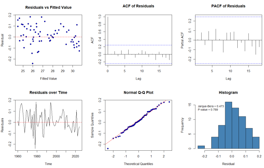
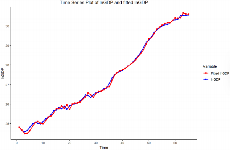
Figure 10 illustrates the comparison of the actual GDP values vs. the fitted values from the ARIMA(1,2,1) model. The shapes of these two curves are very similar and close, indicating that the model fits the trend and patterns of China’s GDP as intended. This evidence further supports the validity of the model.

3.4. Out-of-sample forecasts

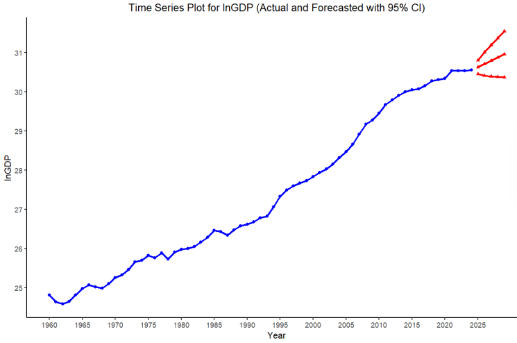
In the preceding section, we determined that the ARIMA (1,2,1) model was appropriate, and we now use it to predict China’s future GDP over the next five years (2025–2029). We used the model equation (6) to predict outside the sample and a 95% confidence interval to help indicate uncertainty in the prediction. Table 3 presents our GDP forecasts for the period 2025–2029.

Figure 11 displays the time series plot of the actual ln(GDP) and the predicted values. The red lines indicate the project path and display the limits of the 95% confidence limits. The forecast suggests GDP is projected to continue to increase in the future, assuming the historical case continues. It is worth noting that these forecasts are model-based forecasts and thus bear the limitations of the ARIMA models. The economic decisions of the future might be affected by unpredictable policy, structural, or external shocks. Thus, while the model serves as a useful reference point, subsequent adjustments will be constantly made as real-world economic developments unfold.

4. Conclusion, limitations and future work

This study utilized the Box-Jenkins method for modeling and forecasting China’s GDP using data from 1960 to 2024 on an annual basis. After conducting stationarity tests and differencing the non-stationary GDP series, the ARIMA(1,2,1) was chosen as the most appropriate model. The decision around the ARIMA specification was evaluated using values of AIC, BIC, and RMSE, which all pointed to the same specifications. Residual diagnostics also confirmed that all assumptions were validated, indicating no significant autocorrelation and assuming the residuals were normally distributed. The model was then used to forecast China’s GDP from 2025 to 2029. There was a noted close alignment between the actual realized and fitted values, and the increase in GDP values in the forecast was clear, as China has sustained GDP growth. Overall, the statistical forecasting approach using the ARIMA(1,2,1) model appears to have captured the underlying dynamic of China’s economic growth, thereby validating the results of this study and demonstrating that ARIMA models can be effectively utilized for short-term economic forecasts.

The ARIMA(1,2,1) model is a good fit for modelling China’s GDP; nevertheless, the study has its constraints. The study only uses univariate time series data and does not consider macroeconomic variables or structural breaks. This makes the ARIMA models less effective in representing potential nonlinearities or abrupt economic changes. Future work could use multivariate models or higher-order forecasting models such as LSTM. Future work could also incorporate high-frequency data to help define better economic dynamics. However, the study offers a useful starting point for any future work in economic time series forecasting.

References

[1]. G. E. P. Box, G. M. Jenkins, G. C. Reinsel, and G. M. Ljung, Time Series Analysis: Forecasting and Control, 5th ed., Wiley, 2015.
[2]. M. R. Abonazel and A. I. Abd-Elftah, “Forecasting Egyptian GDP Using ARIMA Models, ”Reports on Economics and Finance, vol. 5, no. 1, pp. 35–47, 2019.
[3]. F. Mungai, “Modeling and Forecasting Kenyan GDP Using Autoregressive Integrated Moving Average (ARIMA) Models, ”Science Journal of Applied Mathematics and Statistics, 2016.
[4]. B. Maity and B. Chatterjee, “Forecasting GDP Growth Rates of India: An Empirical Study, ”International Journal of Economics and Management Sciences, vol. 1, pp. 52–58, 2012.
[5]. M. N. A. Bhuiyan, K. S. Ahmed, and R. Jahan, “Study on Modeling and Forecasting of the GDP of Manufacturing Industries in Bangladesh, ”Chiang Mai University Journal of Social Science and Humanities, vol. 2, pp. 143–157, 2008.
[6]. A. Uwimana, B. Xiuchun, and Z. Shuguang, “Modeling and Forecasting Africa’s GDP with Time Series Models, ”International Journal of Scientific and Research Publications, vol. 8, pp. 41–46, 2018. https: //doi.org/10.29322/ijsrp.8.4.2018.p7608
[7]. A. Ghazo, “Applying the ARIMA Model to the Process of Forecasting GDP and CPI in the Jordanian Economy, ”International Journal of Financial Research, vol. 12, no. 3, pp. 70–77, 2021.
[8]. R. W. Divisekara, G. J. M. S. R. Jayasinghe, and K. W. S. N. Kumari, “Forecasting the red lentils commodity market price using SARIMA models, ”SN Business & Economics, vol. 1, no. 1, p. 20, 2020.
[9]. P. Mondal, L. Shit, and S. Goswami, “Study of Effectiveness of Time Series Modeling (ARIMA) in Forecasting Stock Prices, ”International Journal of Computer Science, Engineering and Applications, vol. 4, no. 2, pp. 13–21, 2014.
[10]. S. Khan, “ARIMA Model for Accurate Time Series Stocks Forecasting, ”International Journal of Advanced Computer Science and Applications, 2020.
[11]. S. Siami-Namini and A. S. Namin, “Forecasting Economics and Financial Time Series: ARIMA vs. LSTM, ” arXiv preprint, arXiv: 1803.06386, 2018.
[12]. U. M. Sirisha, M. C. Belavagi, and G. Attigeri, “Profit Prediction Using ARIMA, SARIMA and LSTM Models in Time Series Forecasting: A Comparison, ” IEEE Access, vol. 10, pp. 124715–124727, 2022.
[13]. W. Ning, B. Kuan-jiang, and Y. Zhi-fa, “Analysis and Forecast of Shaanxi GDP Based on the ARIMA Model, ”Asian Agricultural Research, vol. 2, pp.34–41, 2010.
Cite this article
Wu,D. (2025). A Comparative Analysis of ARIMA Models for Forecasting China’s GDP. Advances in Operation Research and Production Management,4(2),19-29.
Data availability
The datasets used and/or analyzed during the current study will be available from the authors upon reasonable request.
Disclaimer/Publisher's Note
The statements, opinions and data contained in all publications are solely those of the individual author(s) and contributor(s) and not of EWA Publishing and/or the editor(s). EWA Publishing and/or the editor(s) disclaim responsibility for any injury to people or property resulting from any ideas, methods, instructions or products referred to in the content.
About volume
Journal:Advances in Operation Research and Production Management
© 2024 by the author(s). Licensee EWA Publishing, Oxford, UK. This article is an open access article distributed under the terms and
conditions of the Creative Commons Attribution (CC BY) license. Authors who
publish this series agree to the following terms:
1. Authors retain copyright and grant the series right of first publication with the work simultaneously licensed under a Creative Commons
Attribution License that allows others to share the work with an acknowledgment of the work's authorship and initial publication in this
series.
2. Authors are able to enter into separate, additional contractual arrangements for the non-exclusive distribution of the series's published
version of the work (e.g., post it to an institutional repository or publish it in a book), with an acknowledgment of its initial
publication in this series.
3. Authors are permitted and encouraged to post their work online (e.g., in institutional repositories or on their website) prior to and
during the submission process, as it can lead to productive exchanges, as well as earlier and greater citation of published work (See
Open access policy for details).