1. Introduction:

The field of Earth sciences has long been dedicated to understanding the Earth's internal structure and crustal dynamic processes. The Earth's gravity field serves as a critical data source for studying subsurface material distribution and crustal deformation. However, the Earth's gravity field is influenced by the heterogeneity of subsurface media, resulting in observed gravity anomalies on the Earth's surface. To accurately interpret and understand these anomalies, researchers need to develop new techniques and methods to determine adaptation zones in a data-driven manner.

Data-driven studies of gravity anomaly [1] adaptation zones can assist geologists in better comprehending subsurface geological structures, such as rock types and underground fault zones. This holds significant importance in resource exploration, such as locating and assessing mineral resources, oil and gas reservoirs. Furthermore, research on gravity anomaly adaptation zones can provide information regarding crustal deformation and precursors to seismic activity. This aids in early warning systems for earthquakes and volcanic activity, thereby reducing disaster risks. Understanding subsurface geological conditions is crucial in urban planning and infrastructure development to ensure the safety and stability of buildings and roads. Research on gravity anomaly adaptation zones enables planners to better understand subsurface conditions, leading to more precise planning and design. Research on gravity anomaly adaptation zones contributes to advancing the forefront of Earth sciences, enhancing our understanding of the Earth's internal structure and crustal evolution. This holds significant importance for theoretical research and academic progress.

In summary, data-driven research on gravity anomaly adaptation zones holds importance in multiple fields, including geology, geophysics, resource exploration, seismology, and environmental science. It provides a robust tool for us to better understand the Earth's internal structure and crustal dynamics, thereby aiding in improving resource management, disaster warning, and infrastructure planning. Hence, this paper conducts an in-depth study of gravity anomaly adaptation zones based on factor analysis.

2. Data Collection and Preprocessing

2.1. Data Collection

This paper initially collected data on gravity anomaly values, and the obtained results are as follows:

Table 1: Data on gravity anomaly values

Note: Data sourced from (http://topex.ucsd.edu/)

2.2. Data Preprocessing

Data cleaning in this study primarily involved the following steps:

STEP 1: Inspection of the original data.

STEP 2: Handling missing values and outliers.

STEP 3: Removal of irrelevant variables.

STEP 4: Division of data into regional segments.

Upon conducting the aforementioned STEPs 1 to 3, it was observed that the provided data did not contain any missing values or outliers. Hence, the data was segmented regionally based on the following ranges: Longitude Range: [115.0083, 117.0083], Latitude Range: [9.0045, 11.0068]. The data was grid-based and had a resolution of [resolution]. Consequently, the data was divided into regional sections, the results of which are presented in Table 2:

Table 2

3. Statistical Parameters of Gravity Field Characteristics

Various characteristics of the gravity field describe its changes from different perspectives, serving as essential parameters for selecting adaptation zones. The gravity field data used regional gravity anomaly values, and the following analysis was based on standard grid gravity anomaly values [2].

3.1. Standard Deviation

Standard deviation is a crucial indicator of gravity anomalies and is defined as follows:

where is the grid coordinate

Longitude and latitude standard deviations reflect the fluctuation degrees of gravity anomalies in the respective directions.

In the equation, M represents the number of discrete points in the longitude direction for gravity anomaly values.

The latitude standard deviation reflects the fluctuation dimension of gravity anomalies in the latitude direction. Its definition is as follows:

N denotes the number of discrete points in the latitude direction. While

3.2. Roughness

The roughness of gravity anomaly values in both longitude and latitude directions can be defined as

The absolute roughness of gravity anomalies can be defined as . Here, means square value function and represents the difference function.

3.3. Gradient

The gravity anomaly gradient reflects the extent of changes in gravity anomaly values concerning spatial positions. Generally, the larger the gradient of gravity anomaly values, the richer the spatial information regarding gravity characteristics changes. [3]

The gradients in the longitude and latitude directions for gravity anomalies can be defined separately.

The gradient of gravity anomaly values can be defined as

where represents the mean square value function, represents the difference function, and and denote the longitude and latitude resolutions, respectively.

3.4. Gravity Entropy

Gravity Entropy is a concept commonly used to describe the distribution or clustering degree of geographical spatial data. [4] It is a metric used to measure the uniformity or concentration of data distribution. The definition of gravity entropy is

Here, represents the probability of a specific gravity anomaly value occurrence. And

The longitude and latitude entropy for gravity are defined separately as

where and represent the gravity entropy for each row and column, respectively.

3.5. Plane Correlation

Gravity anomaly plane correlation reflects the correlation of local gravity field features concerning changes in spatial positions of gravity anomaly values. Typically, a larger plane correlation indicates a more pronounced change in gravity field characteristics concerning spatial positions.

The definition of gravity anomaly plane longitude and latitude is as follows:

And the definition of gravity anomaly plane correlation can be expressed as:

In the above equation:

4. Selection of Gravity Adaptation Zones Based on Factors

4.1. Factor Analysis Process

Factor Analysis is a multivariate statistical analysis method used to understand and describe the correlations and structures among variables in observed data. Its main purpose is to reduce the dimensions of multiple observed variables (also known as indicators or items) to identify latent factors or dimensions. These factors are linear combinations of observed variables and can explain the variance-covariance structure of the data. [5] Let the eigenvalue sample data matrix be:

The subsequent step is to establish the factor model of the text:

Here, represents the common factors characterizing all statistical features X of the gravity field, represents the features of X, followed by calculating the sample mean, sample covariance matrix, and sample correlation matrix from the sample data matrix X.

The sample covariance matrix S is defined as:

For the sample correlation matrix

Compute the eigenvalues and standardized eigenvectors, denoted as for eigenvalues and the corresponding unit positive vectors .

Then, solve for the factor loading matrix A of the factor model, selecting the desired factors. Let , () represent the factor loading matrix. Finally, after obtaining the factor loading matrix, derive the determinant of .

4.2. Selection of Adaptation Zones Using Factor Analysis

To visualize the features reflected by the aforementioned parameters of the gravity field, MATLAB software is utilized to plot the distribution of gravity anomaly values and the subdivision of sub-regions, as shown in Figure 1.

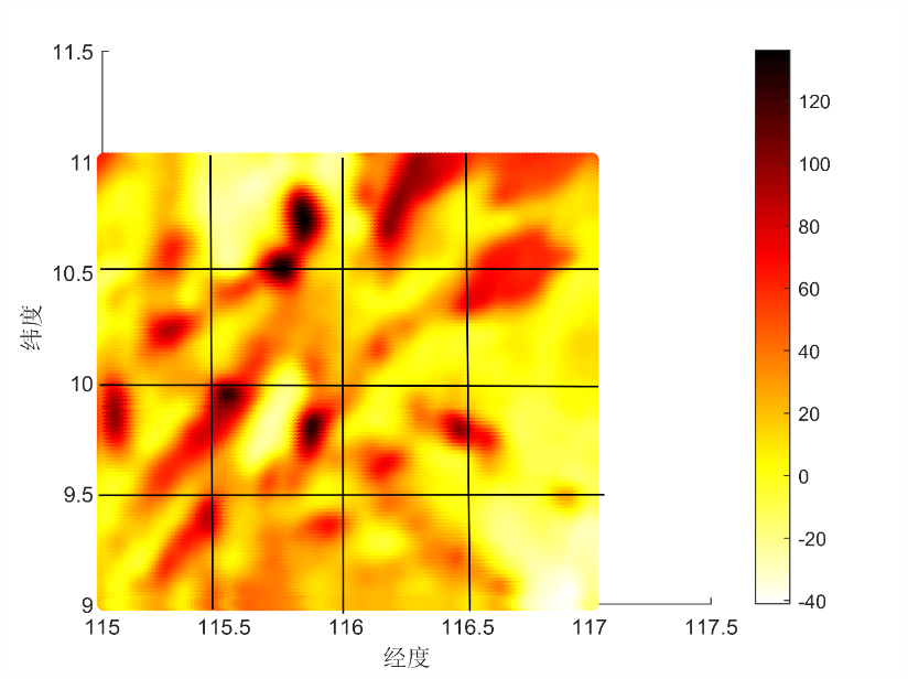
Figure 1. Gravity Anomaly Distribution

Based on the analysis of the above figure, 16 sub-regions were identified. Consequently, adaptive zones were selected based on various characteristics of the gravity regions.

4.3. Result Analysis

Calculation was performed for each of the gravity field characteristic parameters mentioned above. Considering the unit limitations of the characteristics, they were normalized to facilitate subsequent statistical analyses.

Under the aforementioned factor analysis, the results are presented in Table 2:

Table 3: Factor Analysis Results

According to the analysis, these three factors contributed 48.91%, 34.22%, and 10.83%, respectively, to all variables. The cumulative contribution rate reached 91.62%, aligning with practical calculation requirements. Calculations were performed for several sub-regions, eventually obtaining factor scores for 16 sub-regions and their total scores. A comparative curve chart was generated as follows:

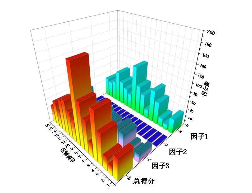
Figure 2. Factor Scores and Total Scores

Higher scores represent higher adaptability in the region, while lower scores indicate lower feasibility for the region as an adaptive zone. Thus, the prioritization of adaptation was determined. Among the 16 sub-regions, sub-regions 5, 6, 7, and 8 exhibited the highest adaptability, sub-regions 1, 4, 12, 13, and 15 showed moderate adaptability, while the remaining sub-regions (2, 3, 6, 10, 11, and 16) demonstrated poor adaptability, resulting in less accurate positioning. MATLAB was employed to create gravity anomaly distribution charts for all sub-regions, as depicted in Figure 3, visualizing the results.

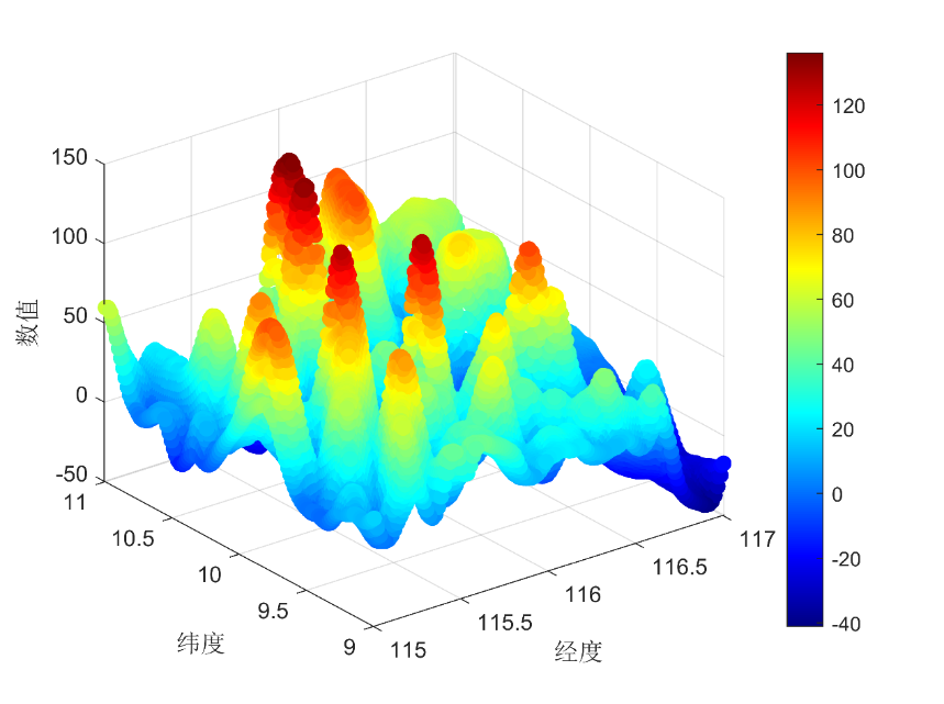
Figure 3 Gravity Anomaly Distribution

5. Conclusion

This paper, concerning the collected data, introduced five statistical parameters for gravity field characteristics. Employing factor analysis facilitated the derivation of factor scores for 16 partitioned sub-regions and vividly presented diverse gravity anomaly distribution charts for different sub-regions. This provides an essential scientific basis for investigating data-driven underwater navigation adaptive zones.

References

[1]. Wang H., Wan X., Richard F. A. Prediction of the South China Sea Seabed Topography Based on Convolutional Neural Networks. Journal of Geodesy and Geodynamics, 1-11 [November 5, 2023].
[2]. Gong J., Zhang C., Zhou X. A Method for Gravity Adaptive Zone Selection Based on Factor Analysis. Journal of Chinese Inertial Technology, 27(06):732-737 [2019].
[3]. Yang F., Shen R., Mei S. Inversion of Emperor Mountain Sea Area Seabed Topography using Joint Gravity Anomaly and Gravity Vertical Gradient Anomaly Data. Acta Oceanologica Sinica, 44(12):126-135 [2022].
[4]. Hu P., Liu J., Zhou X. A New Method for Gravity Field Positioning Based on Eigenvalues. Ship Electronic Engineering, 35(10):58-61 [2015].
[5]. Fu J., Gui S., Yi Q. Source Tracing and Governance Strategies for Soluble Organic Matter in a River in Nanchang City based on Three-Dimensional Fluorescence and Parallel Factor Analysis. Journal of Environmental Engineering, 1-12 [November 5, 2023].
Cite this article
Chen,Q.;Guang,J.;Zhang,L.;Zhang,Y.;Liu,S. (2023). Research analysis of data-driven submarine navigation adaptation zones based on factor analysis. Advances in Operation Research and Production Management,1,5-14.
Data availability
The datasets used and/or analyzed during the current study will be available from the authors upon reasonable request.
Disclaimer/Publisher's Note
The statements, opinions and data contained in all publications are solely those of the individual author(s) and contributor(s) and not of EWA Publishing and/or the editor(s). EWA Publishing and/or the editor(s) disclaim responsibility for any injury to people or property resulting from any ideas, methods, instructions or products referred to in the content.
About volume
Journal:Advances in Operation Research and Production Management
© 2024 by the author(s). Licensee EWA Publishing, Oxford, UK. This article is an open access article distributed under the terms and
conditions of the Creative Commons Attribution (CC BY) license. Authors who
publish this series agree to the following terms:
1. Authors retain copyright and grant the series right of first publication with the work simultaneously licensed under a Creative Commons
Attribution License that allows others to share the work with an acknowledgment of the work's authorship and initial publication in this
series.
2. Authors are able to enter into separate, additional contractual arrangements for the non-exclusive distribution of the series's published
version of the work (e.g., post it to an institutional repository or publish it in a book), with an acknowledgment of its initial
publication in this series.
3. Authors are permitted and encouraged to post their work online (e.g., in institutional repositories or on their website) prior to and
during the submission process, as it can lead to productive exchanges, as well as earlier and greater citation of published work (See
Open access policy for details).