1 Introduction

Efforts to access the efficacy of educational interventions are important for informed decision-making in educational policy and practice. This paper aims to contribute to this discourse by assessing the Average Treatment Effect (ATE) of receiving special education services on the revised Item Response Theory (IRT) scaled math achievement test scores among students. This holds significant implications for educational stakeholders, including policymakers, educators, and researchers, as it provides empirical insights into the potential impacts of these interventions on student academic outcomes.

To achieve this goal, we employ various approaches, each offering unique advantages in estimating the ATE. Specifically, we use conventional techniques linear regression with ordinary least squares (OLS) alongside more advanced methods including propensity score matching (PSM), Bayesian Additive Regression Trees (BART), and Multilayer Perceptron (MLP). These various methods allow a comprehensive examination of the relationship between special education services and math achievement, while accommodating various data distributions and structural complexities inherent in educational datasets.

The analysis is based on data sourced from the Early Childhood Longitudinal Study Kindergarten 2010-11 cohort (ECLS-K:2011), a nationally representative dataset renowned for its longitudinal design and rich socio-demographic variables. Leveraging this dataset, we apply the methods to estimate the ATE of special education services on students' math achievement trajectories, providing an understanding of the intervention's impact across different subgroups and contexts.

Our findings reveal consistently negative ATE results across all modeling approaches, indicating a potential adverse effect of special education services on fifth-grade math scores. This observation emphasizes the complexity inherent in educational interventions and underscores the necessity of critically interrogating their efficacy through robust analysis. To further enhance the validity of our findings, we complement our causal inference and machine learning-based analysis with Principal Component Analysis (PCA), facilitating a comprehensive examination of the underlying data structure and corroborating our conclusions.

By showing the relationship between special education services and math achievement, this research contributes to the broader discourse on educational equity and the intervention effectiveness. Moreover, it emphasizes the importance of method diversity in educational research, advocating for the integration of diverse methods to uncover reveal multifaceted relationships within complex educational datasets. Through these, we try to inform evidence-based decision-making and foster continuous improvement in educational practices aimed at promoting student success and equity.

The remainder of the paper is organized as follows. Section 2 introduces the traditional causal inference and the combination of causal inference and machine learning (ML). Section 3 expounds upon the theoretical underpinnings of various methodologies employed in estimating the average treatment effect of special education service. Section 4 presents the details of the data ECLS-K:2011, and the results of the estimation for the ATE of special education service based on different ML-based methods. Additionally, we employ Principal Component Analysis (PCA) for factor analysis to corroborate our findings. Section 5 encapsulates the paper with concluding remarks, highlighting key insights and avenues for future research.

2 Literature Review

2.1 Traditional causal inference

Causal inference aims to calculate the influence that a modification in a certain variable will have on a desired outcome. The most used models for causal inference are the Rubin Causal Model (RCM) and Causal Diagram [1-6].

Fisher and Neyman each started from the standpoint of statisticians and proposed to discuss causal relationships from the perspective of potential results and randomness [7,8]. Fisher proposed the concept of "randomized controlled trial" (RCT), while Neyman proposed "potential outcomes" and applied them to randomized controlled trials. Rubin further combined the two concepts and systematically proposed the theoretical assumptions, core content and reasoning methods of the potential outcome model [9].

Rubin defines a causal effect: Intuitively, the causal effect of one treatment ( \( t \) ) over control ( \( c \) ) [10]. We consider a framework with \( N \) individuals indexed by \( i \) . \( T_{i}=t \) if a person receives treatment, and \( T_{i}=c \) if not. \( Y_{i}(t) \) denotes person \( i \) ’s outcome when he receives the active treatment and \( Y_{i}(c) \) person \( i \) ’s outcome when he receives the control treatment. The causal effect ( \( τ \) ) of the active treatment the control treatment is given by:

\( τ(X_{i})= Y_{i}(t)- Y_{i}(c) \) (1)

While the problem is that we can never observe both \( Y_{i}(t) \) and \( Y_{i}(c) \) at the same time. Given this, researchers generally concentrate on calculating the Average Treatment Effect (ATE) and Average Treatment Effect on the Treated (ATT) that are specified over N individuals [11,12].

\( τ_{ATE}= E[Y(t)-Y(c)] \) (2)

\( τ_{ATT}=E[Y(t)-Y(c) | T=t \) (3)

Common sample estimands are the Sample Average Treatment Effect (SATE) [13]:

\( \hat{τ_{ATE}}= \frac{1}{N}\sum_{i}[Y_{i}(t)- Y_{i}(c)] \) (4)

Another set of average estimands are the Conditional Average Treatment Effect (CATE) [14]. That is, the expected causal effect of the active treatment for a subgroup in the population:

\( τ_{CATE}= E[Y_{i}(t)X_{i}]- E[Y_{i}(c)X_{i}] \) (5)

Causal models are “mathematical models representing causal relationships within an individual system or population” [15-17]. Causal models can enhance research designs by offering precise guidelines for selecting which variables need to be controlled. They may make it possible to get some answers from the observational data that is already available without the necessity for an interventional investigation. Certain hypothesis cannot be evaluated in the absence of a causal model, which means that certain interventional research is unacceptable for moral or practical reasons. To determine if the findings of one research may be applied to groups that have not been examined, causal models can be helpful. In certain cases, causal models enable the merging of data from several studies to address research concerns that no single data set can address.

2.2 Machine learning and causal inference

Machine learning (ML) spans a diverse array of approaches and applications. Traditional Machine Learning is largely concerned with prediction. It learns a function from the data that can predict an outcome given a collection of input features. Large datasets can be effectively analyzed using it to identify patterns and correlations, but it is not useful for determining the cause-and-effect links between variables. Lately, "Supervised" ML and Deep Learning have evolved beyond prediction-focused applications and ventured into the realm of causal inference [18-23]. The study of causality may be a significant tool in overcoming some of the constraints of correlation-based machine learning systems [23]. Causal inference in machine learning aims at Improving model accuracy and interpretability, which may have significant effects on policy, justice, economics, and health, among other domains. For instance, Causal inference models may be used to account for data biases, comprehend the consequences of actions and policies, and increase the Interpretability and transparency of automated judgments. Classical supervised learning methods includes: (a) regression trees, (b) random forests, (c) boosting, (d) neural networks, and (e) regularized regression (which includes Least Absolute Shrinkage and Selection Operator, or "LASSO," ridge, and elastic net).

3 Methods

In this article, several methods will be included: (a) Linear regression with ordinary least square (OLS), (b) Propensity score matching (PSM, including logistic regression, k-nearest neighbor algorithm), (c) Bayesian Additive Regression Trees (BART), (d) Multi-layer perceptron (MLP).

3.1 OLS

A linear regression with p explanatory variables has the model:

\( Y=β_{0}+\sum_{j=1}^{p}β_{j}X_{j}+ε \) (6)

where Y is the dependent variable, \( β_{0} \) , is the intercept of the model, \( X_{j} \) corresponds to the j-th explanatory variable of the model (j = 1 to p), and \( ε \) is the error term [24]. If \( σ_{j}^{2}=σ^{2} \) (j =1 to p), we can get the estimation of \( β \) by Ordinary Least Square (OLS): \( \underset{β}{min}{\sum_{i=1}^{n}(y_{i}-β_{0}-\sum_{j=1}^{p}β_{j})^{2}}. \) Therefore, we can get the estimation of vector β of the coefficients by \( \hat{β}=(X^{T}X)^{-1}X^{T}Y \) . The vector of the predicted values can be written as follows: \( Y^{*}=X\hat{β}=X(X^{T}X)^{-1}X^{T}Y \) . Otherwise, by the weighted least square, W is a matrix with the \( w_{i}=\frac{1}{σ_{i}^{2}} \) weights on its i-th diagonal [25]. The vector β of the coefficients can be estimated by the following formula \( \hat{β}=(X^{T}WX)^{-1}X^{T}WY \) . The vector of the predicted values can be written as follows: \( Y^{*}=X\hat{β}=X(X^{T}WX)^{-1}X^{T}WY \) .

3.2 PSM

PSM procedure

A Propensity score matching (PSM) is a statistical method used to process data from observational studies [26]. In observational research, there are many data biases and confounding variables due to many complex reasons [27]. To reduce the influence of these biases and confounding variables, PSM selects individuals from the control group who have the same or similar propensity score value as an individual in the treatment group for pairing, to make a reasonable comparison between the experimental group and the control group. PSM is defined as the “propensity” of a person belonging to the treatment group.

\( e(x_{i})=Pr(T_{i}=t | X=x_{i}) \) (7)

The general procedure includes: (i) estimate propensity scores (using logistic regression, random forest etc.). (ii) Match each participant to one or more nonparticipants on propensity score. (iii) Check that covariates are balanced across treatment and comparison groups within strata of the propensity score. (iv) Estimate effects based on new sample [27].

Logistic regression

Logistic regression is a popular classification method, especially when we have binary outcomes, that had been introduced in a variety of books and articles [28,29]. The basic idea is the linear regression method is not accurate for classification problem, so that we need to use logistic regression to give us prediction. For binary outcome \( Y= \begin{cases}0 if No \\ 1 if Yes\end{cases} \) , Logistic regression uses the form: \( Pr{(Y=1X)}= \frac{e^{β_{0}+β_{1}X}}{1+e^{β_{0}+β_{1}X}} \) and \( Pr{(Y=0X)}= \frac{1}{1+e^{β_{0}+β_{1}x}} \) with logit function \( logit(p)=β_{0}+β_{1}X \) . When class K is more than two, \( Pr{(Y=kX)}= \frac{e^{β_{0k}+β_{1k}X_{1}+…+β_{pk}X_{p}}}{\sum_{l=1}^{K}e^{β_{0l}+β_{1l}X_{1}+…+β_{pl}X_{p}}} \) . We can estimate the coefficients by the maximum likelihood estimate (MLE), \( L(β)={\prod_{k=1}^{K}\frac{e^{β_{0k}+β_{1k}X_{1}+…+β_{pk}X_{p}}}{\sum_{l=1}^{K}e^{β_{0l}+β_{1l}X_{1}+…+β_{pl}X_{p}}}} \) [30].

To compute the coefficients, the most popular methods are Newton’s method and quasi-Newton method [31-33]. The basic idea is to repeat the process until the results converges: \( x_{n+1}=x_{n}- \frac{f(x_{n})}{f \\prime (x_{n})} \) . In medical trials, for example, many of the outcome variables are binary. Logistic regression is useful to compute the Average Treatment Effect \( τ_{ATE} \) in the causal inference. Although the average treatment effect cannot be expressed directly in terms of the parameters of the logistic or probit regression model.³³ We can use an indirect method to compute the point estimate for the ATE with a combination of \( β_{0} and β_{1} \) , define as: \( logit^{-1}(β_{0}+β_{1}) - logit^{-1}(β_{1}) \) = \( \frac{e^{β_{0}+β_{1}X}}{1+e^{β_{0}+β_{1}X}} \) - \( \frac{e^{β_{1}X}}{1+e^{β_{1}X}} \) [34].

K-nearest neighbor algorithm

K-nearest neighbor algorithm (KNN) can be used in both regression and classification problems. While in this article, we mainly focused on classification [35]. The goal of KNN is to identify the nearest neighbors of a given query point so that we can assign a class label to that point [36]. The KNN algorithm works by calculating the distances between the query point and all other points in the dataset, typically using Euclidean distance or other distance metrics. Mathematically, the predicted class label \( y \) for a query point \( x \) can be represented as: \( y=model(y_{1}, y_{2}, ..., y_{k}) \) , where \( y_{i} \) represents the class label of the \( i \) th nearest neighbor to the query point, and \( k \) is the number of nearest neighbors to consider (a hyperparameter). The mode function returns the most frequently occurring class label among the \( k \) nearest neighbors.

3.3 BART

The Bayesian Additive Regression Trees (BART) model development process creates a predictive framework through the amalgamation of multiple individual "regression trees" [37]. Regression trees, first introduced in the 1970s, operate by recursively partitioning a set of data into smaller subsets and fitting a constant for each subgroup. However, these individual trees tend to exhibit instability and limited predictive accuracy. BART builds upon this foundation by integrating a “gathering of trees” model with a regularization prior. This approach entails estimating \( E(Y|T,X) \) using a tree, extracting residuals, and then fitting other trees based on the residuals. Such flexibility enables BART to effectively capture interactions and nonlinearities, enhancing its predictive performance. The regularization priors, also referred to as "shrinkage" priors, are equipped with parameters that minimize the influence of each tree on the final model fit. Notably, when BART generates predictions with high accuracy, it becomes instrumental in approximating the average treatment effect by assessing deviations through \( E(Y|T=t) - E(Y|T=c) \) . The Bayesian framework inherent in BART culminates in the generation of a posterior distribution through estimation.

3.4 MLP

Multi-layer perceptron (MLP) is a supplement of feed forward neural network, which is a fully connected multi-layer neural network [38,39]. At the heart of the MLP are its key components: the input layer, hidden layers, and the output layer. Each layer has several neurons that retain numbers ranging from 0 to 1, which are known as activations. The activations in one layer determine the activations in the following layer, connecting with weighted edges. The input layer receives the input signal to be processed, and data flows forward from input to output layer. The output layer in charge of tasks like making predictions of the input or categorizing the input into different groups. The key of the MLP is the hidden layers sandwiched between the input and output layers, which is set before the procedure.

Now we show how activations in layer \( p \) determine the activations in the following layer \( p+1 \) . Suppose there are n neurons on layer \( p \) and m neurons on layer \( p+1 \) . For the j-th neurons \( a_{j}^{p+1} \) in the layer \( p+1 \) , we have \( n \) edges linked it with all the neurons \( a_{i}^{p} \) with weights \( w_{i}^{p} \) (for i from 1 to n). Compute the weighted sum by \( \sum_{i=1}^{n}w_{i}^{p}*a_{i}^{p}-b \) where b is the bias term. Then use activation function like sigmoid \( σ(x)=\frac{1}{1+e^{-x}} or \) \( ReLU(x)=max(0,x) \) to squish this sum into the range between 0 and 1. To get the optimal set of coefficients, backpropagation is a vital training algorithm. It comprises a forward pass, where input data produces predictions, and a backward pass, where errors are propagated backward to adjust weights and biases. During the backward pass, gradients are calculated, representing the sensitivity of the network's output to changes in its parameters. These gradients guide the iterative update of weights and biases using optimization algorithms like gradient descent. The process allows the network to learn from errors and improve its performance over multiple training iterations, enabling it to generalize well to new data.

4 Data Analysis

4.1 Data description

In this article, we selected data from the Early Childhood Longitudinal Study Kindergarten 2010-11 cohort (ECLS-K:2011). The kindergarten class of 2010-11 cohort is a sample of children followed from kindergarten through the fifth grade, released by the National Center for Education Statistics within the Institute of Education Sciences (IES) of the U.S. Department of Education. Insights into children's cognitive, social, emotional, and physical development are gleaned from inputs provided by children themselves, their families, educators, schools, and caregivers.

The data are washed from the raw data. The data used in analysis include 7362 individuals, with 429 “treated” subjects (receiving Special Education Services) and 6933 controls. The exposure variable (Special Education Services) is a binary variable F5SPECS, which \( F5SPECS=1 \) if subjects received treatment, \( F5SPECS=0 \) if not. The outcome variable (Fifth Grade Math Score) is continuous, ranging from 50.9 to 170.7. Other relevant variables include six aspects: Demographic, Academic, family context, Health, Parent rating of child, which contains 30 variables to measure the child from a variety of aspects.

4.2 Model comparison

Since we can’t observe a child’s math score both received special education service and not received, then we need to estimate the score .We use four models: Ordinary Least Square regression (OLS), Propensity Score Matching (PSM), Bayesian Additive Regression Trees (BART), Multi-layer perceptron (MLP), to calculate the estimate average treatment effect (ATE) of Special Education Service on the Fifth Grade Math Score, with data from ECLS-K:2011.

The training data is the given data above, and the testing data is created by replacing the exposure variable F5SPECS to its contradiction, 0 to 1 or 1 to 0. Then, we can get the estimate of outcomes through models. Now we have two columns of outcomes, one is the given data, the other is the estimands. To compute ATE, we sum the outcomes that received treatment, and minus the summation of outcomes without treatment, then divide by the number of individuals.

Table 1. Model Comparison

The results are shown in Table 1 above. The table show that all models give negative ATE results, which means the Special Education Services have negative effect on Fifth Grade Math Score for students. The variance for OLS is the highest. While, for ML-based approaches, BART perform better in this scenario. It has a high R squared and meanwhile a lower variance. While PSM perform not so well. Since the R-squared of PSM won’t tell much useful information, so we mainly focus on the confidence interval, which is also much larger than others. For MLP, it doesn’t perform well under these circumstances.

4.3 Factor analysis

Figure 1 shows the result of correlation matrix. The stronger the positive correlation between the two variables, the higher the value. They are most negatively correlated when the value is nearer -1.

Then we conduct Principal Component Analysis (PCA) to the data. The significance of each principal component is shown in figure 2, which may also be used to calculate how many principal components to preserve. 46.7% of the total variance can be explained by the first principal component. This suggests that the first principal component alone can capture more than half of the data in the collection of 32 variables. Approximately 90% of the variance may be explained by the cumulative percentage of Comp.1 to Comp.14. This indicates that the data can be accurately represented by the first fourteen principal components.

The next step is to find the amount that each variable is represented in each component. The square cosine is represented by a quality of representation known as the Cos2. A low value indicates that the variable isn't fully captured by that element, whereas a high value suggests an effective representation of the variable within that component. From figure 3, MIRT, outcome, WK5ESL, RIRT, are the top four variables with the highest cos2, hence contributing the most to PC1 to PC14.

The biplot and attributes importance can be combined to create a single biplot, where attributes with similar cos2 scores will have similar colors. From figure 5, all the variables grouped together exhibit positive correlations. While variables with negative correlations are positioned on opposite sides of the biplot's origin. The farther a variable is from the origin, the more effectively it is represented. High cos2 attributes are colored in green: MIRT, outcome, WKSESL and RIRT. Mid cos2 attributes have an orange color: P1HMAFB, P1FSTAMP, WKWHITE, S2KMINOR, approachT1, P1SOLVE, C1FMOTOR, ONEPARENT, P1HSEVER, P1ATTENI, treatment and P1PRONOU. Finally, low cos2 attributes have a black color: wt_ounces, P1IMPULS, P1EARLY, S2KPUPRI, Р1EXPECT, PINUMSIB, PIAGEENT, PIFIRKDG, STEPPARENT, C1GMOTOR, chg14, GENDER, P1SADLON, P1DISABL, P1HSCALE, WKCAREPK.

We can find that Kindergarten Math Score, Reading Score, Approaches to Learning Rating and Fine Motor Skills are positively relate to the Fifth Grade Math Score. On the other hand, Attentive, Problem Solving, Verbal Communication and Special Education Services have negative effect on the Fifth Grade Math Score, which is inconsistent with common sense [40,41]. However, this result matches with what we have got through causal inference and ML-based methods.

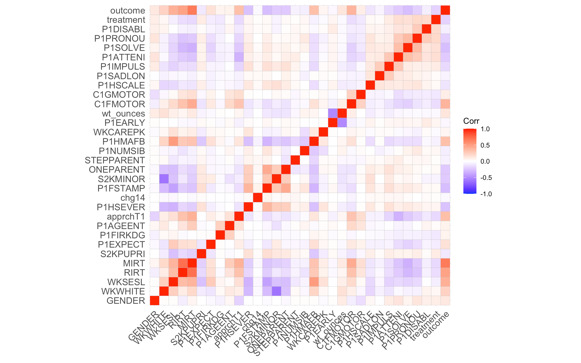
Figure 1. Correlation Plot

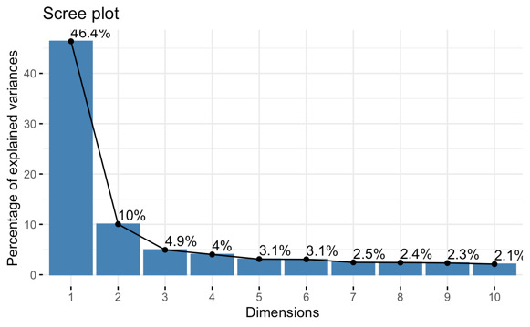
Figure 2. Scree Plot

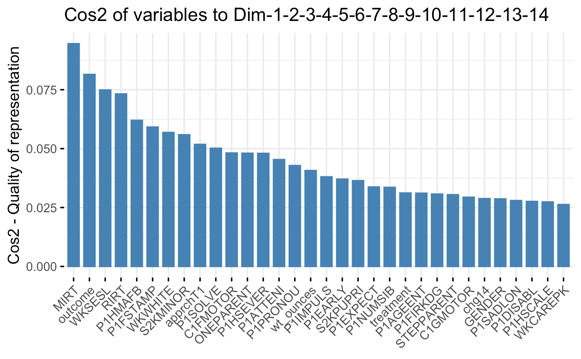
Figure 3. Contribution of Each Variable

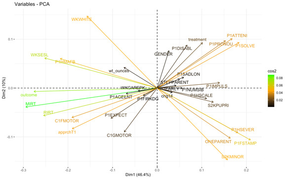
Figure 4. Biplot Combined with cos2

5 Conclusions

Based on the findings derived from our experimental analysis, several key conclusions emerge. Firstly, our results show a negative impact of Special Education Services on Fifth Grade Math Scores. This emphasizes the importance of critically evaluating the efficacy of educational interventions, particularly within the domain of special education.

Moreover, our comparative analysis highlights the efficacy of machine learning (ML)-based methodologies in reducing bias when estimating the average treatment effect. Particularly the substantial reduction in bias observed compared to more traditional methods. However, despite these advancements, there remains considerable room for improvement within our study.

Specifically, our analysis reveal that the methods employed do not consistently yield accurate estimates of the average treatment effect, with several models exhibiting relatively large variances. Notably, the performance of deep learning methods appears suboptimal in this context. Possible explanations for this discrepancy include insufficient sample sizes within the dataset or suboptimal configurations of key parameters such as loss function, mini-batch size, and activation functions.

Considering these limitations, future research endeavors should prioritize addressing these methodological challenges to enhance the robustness and generalizability of findings within health services research. Furthermore, it is important to recognize the evolving role of machine learning in facilitating causal inference within the realm of health services research. The combination of machine learning and causal inference holds immense promise for advancing our understanding of complex phenomena and informing evidence-based decision-making in healthcare policy and practice. As such, the integration of these approaches promises transformative advances in the field, heralding a new era of data-driven insights and interventions designed to advance health equity and improve subject outcomes.

References

[1]. Rubin, D. B. (1974). Estimating causal effects of treatments in randomized and nonrandomized studies. Journal of educational Psychology, 66(5), 688.
[2]. Rubin, D. B. (1977). Assignment to treatment group on the basis of a covariate. Journal of educational Statistics, 2(1), 1-26.
[3]. Rubin, D. B. (1978). Bayesian inference for causal effects: The role of randomization. The Annals of statistics, 34-58.
[4]. Rubin, D. B. (1980). Randomization analysis of experimental data: The Fisher randomization test comment. Journal of the American statistical association, 75(371), 591-593.
[5]. Rubin, D. B. (2005). Causal inference using potential outcomes: Design, modeling, decisions. Journal of the American Statistical Association, 100(469), 322-331.
[6]. Pearl, J. (2018). Theoretical impediments to machine learning with seven sparks from the causal revolution. arXiv preprint arXiv:1801.04016.
[7]. Fisher, R. A. (1956). Statistical methods and scientific inference.
[8]. Splawa-Neyman, J., Dabrowska, D. M., & Speed, T. P. (1990). On the application of probability theory to agricultural experiments. Essay on principles. Section 9. Statistical Science, 465-472.
[9]. Pearl, J., & Shafer, G. (1995). Probabilistic reasoning in intelligent systems: Networks of plausible inference. Synthese-Dordrecht, 104(1), 161.
[10]. Holland, P. W. (1986). Statistics and causal inference. Journal of the American statistical Association, 81(396), 945-960
[11]. Abadie, A., Angrist, J., & Imbens, G. (2002). Instrumental variables estimates of the effect of subsidized training on the quantiles of trainee earnings. Econometrica, 70(1), 91-117.
[12]. Imbens, G. W. (2004). Nonparametric estimation of average treatment effects under exogeneity: A review. Review of Economics and statistics, 86(1), 4-29.
[13]. Imbens, G. W., & Rubin, D. B. (2015). Causal inference in statistics, social, and biomedical sciences. Cambridge university press.
[14]. Rosenbaum, P. R., & Rubin, D. B. (1983). The central role of the propensity score in observational studies for causal effects. Biometrika, 70(1), 41-55.
[15]. Hitchcock, C. (2020). Communicating causal structure. In Perspectives on Causation: selected papers from the Jerusalem 2017 workshop (pp. 53-71). Springer International Publishing.
[16]. Prosperi, M., Guo, Y., Sperrin, M., Koopman, J. S., Min, J. S., He, X., ... & Bian, J. (2020). Causal inference and counterfactual prediction in machine learning for actionable healthcare. Nature Machine Intelligence, 2(7), 369-375.
[17]. Pearl, J. (2019). The seven tools of causal inference, with reflections on machine learning. Communications of the ACM, 62(3), 54-60.
[18]. Grimmer, J. (2015). We are all social scientists now: How big data, machine learning, and causal inference work together. PS: Political Science & Politics, 48(1), 80-83.
[19]. Athey, S. (2015, August). Machine learning and causal inference for policy evaluation. In Proceedings of the 21th ACM SIGKDD international conference on knowledge discovery and data mining (pp. 5-6).
[20]. Hair Jr, J. F., & Sarstedt, M. (2021). Data, measurement, and causal inferences in machine learning: opportunities and challenges for marketing. Journal of Marketing Theory and Practice, 29(1), 65-77.
[21]. Ramachandra, V. (2018). Deep learning for causal inference. arXiv preprint arXiv:1803.00149.
[22]. Kreif, N., & DiazOrdaz, K. (2019). Machine learning in policy evaluation: new tools for causal inference. arXiv preprint arXiv:1903.00402.
[23]. Pearl, J. (2018). Theoretical impediments to machine learning with seven sparks from the causal revolution. arXiv preprint arXiv:1801.04016.
[24]. Montgomery, D. C., Peck, E. A., & Vining, G. G. (2021). Introduction to linear regression analysis. John Wiley & Sons.
[25]. Schaffrin, B., & Wieser, A. (2008). On weighted total least-squares adjustment for linear regression. Journal of geodesy, 82, 415-421.
[26]. Caliendo, M., & Kopeinig, S. (2008). Some practical guidance for the implementation of propensity score matching. Journal of economic surveys, 22(1), 31-72.
[27]. Abadie, A., & Imbens, G. W. (2016). Matching on the estimated propensity score. Econometrica, 84(2), 781-807.
[28]. Sperandei, S. (2014). Understanding logistic regression analysis. Biochemia medica, 24(1), 12-18.
[29]. Pregibon, D. (1981). Logistic regression diagnostics. The annals of statistics, 9(4), 705-724.
[30]. Gourieroux, C., & Monfort, A. (1981). Asymptotic properties of the maximum likelihood estimator in dichotomous logit models. Journal of Econometrics, 17(1), 83-97.
[31]. Moré, J. J., & Sorensen, D. C. (1982). Newton's method (No. ANL-82-8). Argonne National Lab.(ANL), Argonne, IL (United States).
[32]. Berahas, A. S., Bollapragada, R., & Nocedal, J. (2020). An investigation of Newton-sketch and subsampled Newton methods. Optimization Methods and Software, 35(4), 661-680.
[33]. Schmidt, M., Kim, D., & Sra, S. (2011). Projected Newton-type methods in machine learning.
[34]. Kent, D. M., & Hayward, R. A. (2007). Limitations of applying summary results of clinical trials to individual patients: the need for risk stratification. Jama, 298(10), 1209-1212.
[35]. Guo, G., Wang, H., Bell, D., Bi, Y., & Greer, K. (2003). KNN model-based approach in classification. In On The Move to Meaningful Internet Systems 2003: CoopIS, DOA, and ODBASE: OTM Confederated International Conferences, CoopIS, DOA, and ODBASE 2003, Catania, Sicily, Italy, November 3-7, 2003. Proceedings (pp. 986-996). Springer Berlin Heidelberg.
[36]. Zhang, M. L., & Zhou, Z. H. (2007). ML-KNN: A lazy learning approach to multi-label learning. Pattern recognition, 40(7), 2038-2048.
[37]. Chipman, H. A., George, E. I., & McCulloch, R. E. (2010). BART: Bayesian additive regression trees.
[38]. Gardner, M. W., & Dorling, S. R. (1998). Artificial neural networks (the multilayer perceptron)—a review of applications in the atmospheric sciences. Atmospheric environment, 32(14-15), 2627-2636.
[39]. Popescu, M. C., Balas, V. E., Perescu-Popescu, L., & Mastorakis, N. (2009). Multilayer perceptron and neural networks. WSEAS Transactions on Circuits and Systems, 8(7), 579-588.
[40]. Cimpian, J. R., Lubienski, S. T., Timmer, J. D., Makowski, M. B., & Miller, E. K. (2016). Have gender gaps in math closed? Achievement, teacher perceptions, and learning behaviors across two ECLS-K cohorts. AERA Open, 2(4), 2332858416673617.
[41]. Little, M. (2017). Racial and socioeconomic gaps in executive function skills in early elementary school: Nationally representative evidence from the ECLS-K: 2011. Educational Researcher, 46(2), 103-109.
Cite this article
Li,L. (2024). Assessing the Causal Effect of Special Education Services on Math Achievement: A Causal Inference and Machine Learning Study. Advances in Social Behavior Research,7,20-27.
Data availability
The datasets used and/or analyzed during the current study will be available from the authors upon reasonable request.
Disclaimer/Publisher's Note
The statements, opinions and data contained in all publications are solely those of the individual author(s) and contributor(s) and not of EWA Publishing and/or the editor(s). EWA Publishing and/or the editor(s) disclaim responsibility for any injury to people or property resulting from any ideas, methods, instructions or products referred to in the content.
About volume
Journal:Advances in Social Behavior Research
© 2024 by the author(s). Licensee EWA Publishing, Oxford, UK. This article is an open access article distributed under the terms and
conditions of the Creative Commons Attribution (CC BY) license. Authors who
publish this series agree to the following terms:
1. Authors retain copyright and grant the series right of first publication with the work simultaneously licensed under a Creative Commons
Attribution License that allows others to share the work with an acknowledgment of the work's authorship and initial publication in this
series.
2. Authors are able to enter into separate, additional contractual arrangements for the non-exclusive distribution of the series's published
version of the work (e.g., post it to an institutional repository or publish it in a book), with an acknowledgment of its initial
publication in this series.
3. Authors are permitted and encouraged to post their work online (e.g., in institutional repositories or on their website) prior to and
during the submission process, as it can lead to productive exchanges, as well as earlier and greater citation of published work (See
Open access policy for details).