1. Introduction

Economic recessions are generally characterized by a widespread and substantial decrease in economic performance, persisting for an extended period, often more than a few months. This downturn is observable in multiple economic measures such as Gross Domestic Product (GDP), income, employment rates, industrial output, and the volume of sales in wholesale and retail. Typically, a prevalent method to recognize a recession is the occurrence of two successive quarters of declining GDP.

The COVID-19 pandemic has brought both immediate effects and ongoing consequences on the U.S. economy. The COVID-19 pandemic significantly affects the economics of healthcare systems. The immediate demands of handling the pandemic have already led to considerable financial strain (Cater et al., 2020) [1]. Temporary adverse supply shocks induced by the COVID-19 lead to a decrease in both production and employment (Guerrieri et al., 2020) [2]. The real GDP of the United States for the whole year of 2020 decreased by 3.5% compared to the previous year. This is the first time that the GDP in the United States has declined since the end of the financial crisis in 2009, and the decline is the largest since World War II. In mid-March 2020, individuals with higher incomes significantly reduced their spending, particularly in areas with high COVID-19 infection rates and in sectors requiring in-person interaction. This reduction in expenditure led to a substantial decrease in the revenue of small businesses in affluent postal code areas. These businesses, facing financial strain, laid off many employees, resulting in widespread unemployment, especially among low-wage workers in wealthier regions (Chetty et al., 2020) [3]. The COVID-19 pandemic rapidly escalated, dramatically impacting the United States. As an illustration, the unemployment rate in the U.S. was 3.5% in February 2020, matching the lowest level in 67 years. However, just six weeks after, the situation changed drastically: Almost ten million U.S. citizens applied for unemployment benefits over a two-week period (Chaney & Morath, 2020) [4]. The COVID-19 catastrophe will lead to a significant reduction in output, with over half of this decline attributed to economic uncertainty caused by COVID-19 (Baker et al., 2020) [5]. The economic performance of the United States after the pandemic from the perspectives of GDP, income, employment and output can tell the U.S. economy has experienced economic recessions.

In the post pandemic era, considering the uncertainty caused by the COVID-19 pandemic, this article considers multiple machine learning models to forecast GDP and predict future macroeconomics. Firstly, this study begins by examining the relationship between the COVID-19 pandemic and economic mobility, thereby elucidating the pandemic’s impact on the economy. Subsequently, it delves into machine learning models, utilizing various models to predict the GDP. A comparative analysis of the results from these models is conducted to identify the most suitable one. In the process of model selection, the chosen model will also be used to forecast the GDP of other regions, ensuring a more careful and appropriate choice of model for GDP forecasting.

2. The Covid-19 Pandemic and Economic Recession

The spread of the COVID-19 pandemic was remarkably fast, prompting governments worldwide to adopt lockdown policies to reduce infection rates. These policies aimed to decrease contact between individuals, thereby curbing the transmission and spread of the virus. There was a notable reduction in the growth rate and an extension in the doubling time of cases as a result of the lockdown measures implemented (Lau et al., 2020) [6]. Stricter restrictions on movement in high-risk areas appear to have the capability to decelerate the transmission of COVID-19. Such measures, while reducing interactions among people, led to a decrease or lower efficiency in economic activities within communities, resulting in reduced community income. Evaluating these policies becomes more complex due to individual behavior changes (also known as community responses) that occur independently of government actions. A substantial amount of economic research shows that individuals tend to react logically to information, altering their decisions and behaviors in response to health and various other risks (Mendolia et al., 2021) [7]. Taking Italy as an example, the liquidity changes brought about by the COVID-19 pandemic have a greater impact on towns with higher fiscal capacity, leading to an exacerbation of poverty and inequality. In regions with lower per capita income, the mobility contraction is stronger (Bonaccorsi et al., 2020) [8]. Meanwhile, the correlation analysis of Indonesia revealed a significant association between the pandemic, marked by COVID-19 positive cases, and mortality rates in relation to conditions including socio-economic factors, displaying an average correlation coefficient exceeding 0.80 (Prawoto et al., 2020) [9]. To understand the relationship between economic mobility and COVID-19, the correlation analysis can give an idea of community mobility of U.S. during the pandemic.

2.1. Backgrounds of the Pandemic in US, 2020

The outbreak of the pandemic has negatively impacted socio-economic performance in multiple ways. Firstly, the global supply chain was disrupted for an extended period due to restrictions on transportation. This not only stalled global economic development but also led to border closures in many countries, hindering the exchange of resources, especially scarce items like medical equipment and medicines, thereby exacerbating the pandemic's impact. Secondly, trade restrictions imposed by countries due to the pandemic caused a decline in global trade volume, a reduction in output for various businesses, and a decrease in employment rates. Lastly, the financial markets experienced severe turbulence. In addition to the economic losses caused by the pandemic, the global investors' panic led to a loss of market confidence, further driving the economy into recession. The U.S. plays an important role in economy all over the world and is also damaged by the COVID-19.

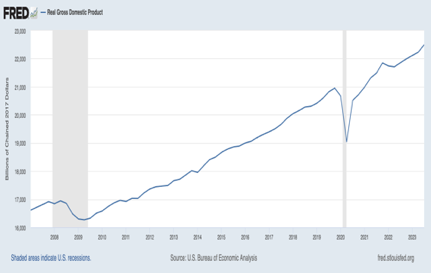
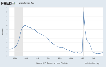
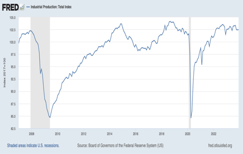
(b) (c)

Figure 1. (a) U.S. Real GDP, (b) Unemployment Rate and (c) Industrial Production. Source: Federal Reserve Bank of St. Louis

From the perspective of stock market, the recovery of the US economy does not depend on macroeconomics, but on the control of the epidemic (Thorbecke, 2020) [10].

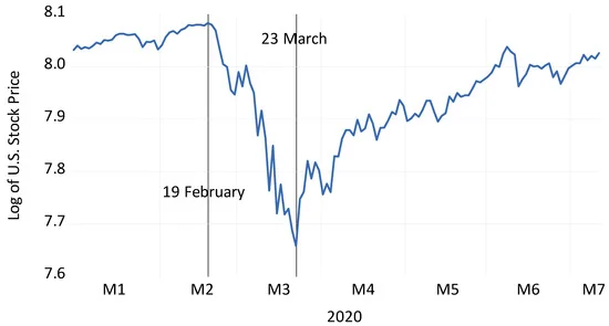
Figure 2. U.S. aggregate stock prices. Source: Datastream database.

2.2. Economic Mobility Data

The study of the relationship between community mobility and the Covid-19 pandemic is based on the data of COVID-19 Community Mobility Report from Google.

Table 1. The community mobility variables

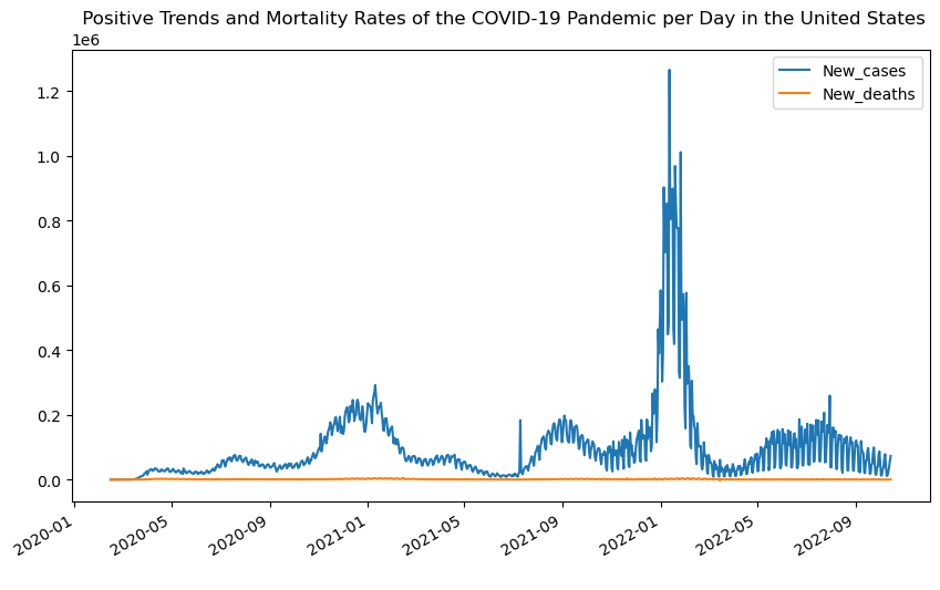
Figure 3. Positive Trends and Mortality Rates of the COVID-19 Pandemic per Day in the United States

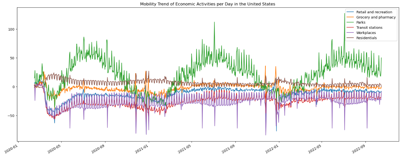
Figure 4. Mobility of Economic Activities per Day in the United States

The figure can show that the pandemic began in the January 2020 and the first peak of daily new cases happened in January 2021, which was a long period. As the figure 3 shows, the highest peak happened in January 2022. The mobility trend for the workplace and the mobility trend for places including all kinds of parks were low as the figure 4 shows, which is interesting because they could match to the peak of pandemic.

At the beginning of COVID-19, in the first half of 2020, these variables related to community mobility were greatly affected. Except for the variables of residences, other factors declined significantly. In the long run, although these factors are gradually stabilizing now, they still cannot return to the level before the outbreak of the epidemic.

2.3. Correlation Analysis

After WHO announced the COVID-19 epidemic, governments gradually implemented strict stay-at-home orders and social restrictions. In the United States, such policies have gone through multiple stages of easing and tightening, mainly due to the following two factors. Firstly, vaccine variants. For example, in mid-2020, the growth in the number of positive COVID-19 cases gradually slowed down, and state governments also relaxed their home stay restrictions. However, due to the Alpha variant in the second half of 2020, the number of positive COVID-19 cases surged to a small peak in January 2020 and the policy of staying at home has been tightened. Secondly, the vaccine has not been popularized, making it difficult to control the COVID-19 epidemic. For example, on December 11, 2020, the emergency use authorization application of Pfizer COVID-19 vaccine was approved by the Food and Drug Administration, allowing the vaccine to be used for people aged 16 and above. In May 2021, the FDA expanded the scope of emergency use authorization for this vaccine, which could be used urgently for people aged 12 to 15. The Moderna COVID-19 vaccine was officially approved by the European Commission on January 6, 2021. But at the end of 2021, the number of infected individuals grew rapidly and reached its peak in January 2022.

Table 2. Correlations between COVID-19 and Community Mobility in the United States

Table 2 displays the correlation coefficient calculations between the pandemic and economic mobility across various sectors—imcluding 6 sectors such as residential areas sector, workplaces sector, transit stations sector, parks sector, grocery and pharmacy sector and retail and recreation sector—within the United States during 2/15/2020-10/15/2022. From Table 2, it can be showed that RAC, GAP, PAR and TRS are negatively correlated with NEC, implying that the Covid-19 brought negative effects on economic mobility across sectors of RAC, GAP, PAR and TRS. The correlation between RES and NEC is positive at the 0.05 significance level, which means people should stay at home to decrease the positive cases of COVID-19.

The new death cases also significantly correlated with economic mobility. NED is negatively related with RAC, GAP, PAR, TRS and WOR, also implying that the Covid-19 brought negative effects on economic mobility across sectors of RAC, GAP, PAR, TRS and WOR. Only RES is positively related with NED, which means economic mobility within residentials could help to decrease the new death cases.

The main emphasis lies in containment, treating the sick, and assisting communities in dealing with the epidemic. The affected countries may face a substantial potential income loss, leading to a global GDP decline of up to 3.9% (Maliszewska et al., 2020) [11].

3. Predictive Models

The pandemic and COVID-19 have had a huge impact on every part of people’s life. Numerous nations are experiencing economic disruptions because of the pandemic. However, the harm is not irreversible, and global societies can overcome this setback through collaborative efforts across all aspects of life (Alsolami et al., 2021) [12]. Since March 2020, the global impact of the COVID-19 pandemic on both the world and economy has been severe. In April, the unemployment rate in the United States surged to 14.7%, with personal consumption expenditures dropping by nearly 20% compared to the February peak. The economy in the United States has been severely affected. Industries like entertainment and aviation faced widespread stagnation in various parts of the country. Compared with the historical disasters happened in the United States, the Covid-19 might bring even more pessimistic outcomes. (Ludvigson et al.,2020) [13]. Predicting the future macroeconomic effects of the pandemic is essential for guiding appropriate policy responses and aiding decision-making for businesses and households (Primiceri & Tambalotti, 2020) [14]. Even if the predictions are based on many assumptions, this undertaking is expected to yield valuable insights into the origins of economic fluctuations and how they spread across different sectors and over time in the economy.

3.1. Data

From the FRED, 12 variables related to the US economy are collected. GDP is chosen as the dependent variable to show the development of the economy and other 11 variables such as unemployment rate, CPI, PPI and so on are chosen to be the independent variables.

Table 3. Economic variables in the United States

3.2. Models

3.2.1. Vector Autoregressive Model

The Vector Autoregressive (VAR) Model is a statistical method employed in time series analysis and econometrics. It concurrently models several variables by expressing each variable as a linear combination of its prior values and the preceding values of other variables in the system (Sims, 1980) [15]. VAR models are beneficial for predicting and comprehending the interconnections among various time series variables, making them valuable in economic and financial analyses.

A VAR with p lags can be written as:

\( y_{t}=c+A_{1}y_{t-1}+A_{2}y_{t-2}+…+A_{p}y_{t-p}+e_{t} \ \ \ (1) \)

\( y_{t-i} \) : the ith lag of \( y_{t} \)

\( c \) : the constant as the intercept of the model (k-vector)

\( A_{i} \) : a time-invariant matrix (k*k)

\( e_{t} \) : error terms (k-vector)

Besides, the error terms should satisfy the following conditions:

\( E(e_{t})=0\ \ \ (2) \)

\( E(e_{t}e^{ \prime }_{t})=Ω\ \ \ (3) \)

\( E(e_{t}e^{ \prime }_{t-k})=0\ \ \ (4) \)

3.2.2. Machine Learning Models

By learning patterns of data, repetitive tasks can be automatically completed, thereby improving work efficiency and accuracy, so it can be more efficient to predict the economy by applying the Machine Learning (ML) models. Besides, to better train the model, the feature extraction method involving converting raw data into a set of numerical features, diminishing dimensionality while preserving essential information is also applied to select proper features (Guyon & Elisseeff, 2006) [16].

(1) Support Vector Machines model

Support Vector Machines (SVMs) are supervised machine learning models used for classifying and regressing data. They identify a hyperplane in the feature space to distinguish between different classes, with support vectors being the closest data points to this boundary. Well-suited for high-dimensional spaces, SVMs employ a kernel trick to handle intricate relationships by transforming features. Found in applications like image and text classification, as well as financial forecasting, SVMs are valued for their robustness and versatility across diverse domains.

Linear SVM: Vapnik (1963) [17] initialed maximum-margin hyperplane technique created a linear classifier. Given a training dataset \( (x_{1,}y_{1}),…,(x_{n,}y_{n}) \) , \( y_{i} \) is either 1 or -1, which is used to indicate the class to the which \( x_{i} \) is, and \( x_{i} \) is a real vector (p-dimensional). The hyperplane that divides the group of points is defined as a set of points x satisfying:

\( w^{T}x-b=0\ \ \ (5) \)

w: normal vector (not necessarily) to the hyperplane

\( \frac{b}{‖w‖} \) : the distance by which the hyperplane is shifted from the origin along the normal vector w.

What’s more, the maximum-margin hyperplane is what we want to find so that the distance between the \( x_{i} \) (the nearest point) from each group can be maximized.

Nonlinear SVM: Boser et al. (1992) [17] developed a method of applying the kernel trick — first put out by Aizerman et al. (1964) [18] — to maximum margin hyperplanes to produce nonlinear classifiers. The nonlinear kernel function is used to replace the dot product. Even when operating in a higher-dimensional feature space, which raises the generalization error of support vector machines, the nonlinear approach could perform well.

(2) XGBoost model

XGBoost (eXtreme Gradient Boosting) is a popular ML method that is commonly used for complex regression and various classification problems. As a kind of the gradient boosting framework, it can use various methods including ensemble learning, regularization, parallelization, tree pruning, and automatic handling of missing variables to produce accurate and useful prediction models. Besides, this model has great efficiency with its high speed.

(3) LightGBM model

LightGBM (light gradient-boosting machine) is also a kind of gradient boosting framework, which is widely used to effectively train the big datasets. It applies the main idea of a leaf-wise tree growth technique for faster training and focuses on classification and regression application. As a member of gradient boosting framework, it is also well-known for its speed and scalability (Brownlee,2020) [19], which can handle large datasets in a variety of machine learning applications.

(4) Deep learning methods (LSTM network)

As a method to build the forecast model, the deep learning method also plays an important part in the machine learning system. The Long short-term memory (LSTM) network is a type of recurrent neural network (RNN) which is developed to deal with prolonged dependencies in time series. This model applied memory cells and gated mechanisms so that the model can understand complex patterns, thereby making the model ideally suited for undertakings including natural language processing and time series predictions. (Memory, 2010) [20]

3.3. Results

3.3.1. Vector Autoregressive Model

By applying the VAR model, two models including var (12) with lowest AIC and var (2) with lowest BIC are presented in the following table.

Table 4. Results of VAR model

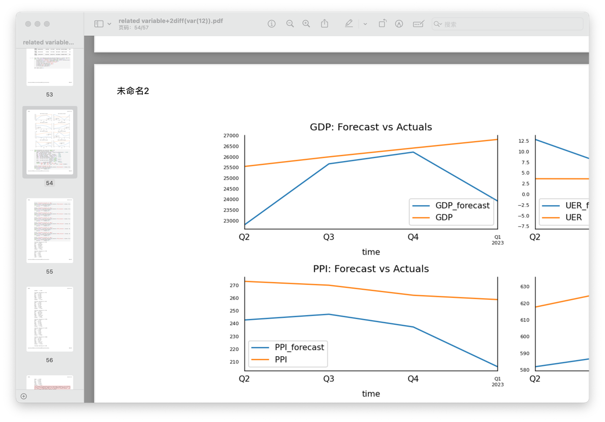
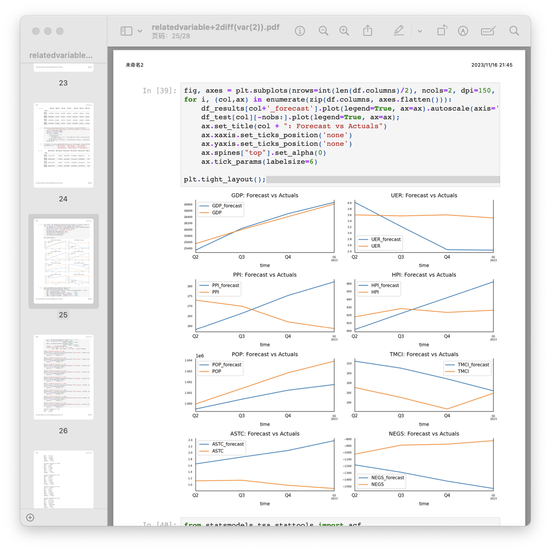
Figure 5. Model selected by AIC (var (12)), Model selected by BIC (var (2))

The AIC-selected model appears to have higher values according to accuracy compared to the BIC-selected model, indicating a potential trade-off between model complexity (captured by AIC) and goodness of fit (captured by BIC). MAPE, MAE, and RMSE provide insights into the accuracy of GDP forecasts. Lower values are generally desired for these metrics, indicating better predictive performance. The correlation values (0.3423 for AIC and 0.9925 for BIC) with the actual GDP suggest the strength of the relationship captured by each model. A higher correlation indicates a better fit. Besides, the MINMAX reflects the difference between predicted and actual values, and the model of var (2) selected by BIC has lower outcome, which means the outcomes and predictions are closer. Both models have advantages and disadvantages, so further study is needed to forecast the economy in the United States.

3.3.2. Machine Leaning Model

From the results of feature selection, 7 variables with score>1 including UER, POP, T1YM, ASTC, NEGS, PSR and SPPE are chose by the model of feature extraction, which means in the machine process of forecasting future economy of the United States with the dependent variable GDP, the independent variables are Unemployment Rate, Population, 1-Year Treasury Constant Maturity Minus Federal Funds Rate, Moody's Seasoned Aaa Corporate Bond Yield Relative to Yield on 10-Year Treasury Constant Maturity, Net Exports of Goods and Services, Personal Saving Rate and S&P 500 PE Ratio.

Table 5. Feature extraction scores (the United States)

By using the result of feature selection, the SVMs model, XGBoost model, LightGBM model and LSTM network are trained. The results are as followed.

Table 6. Machine learning results

According to the results, XGBoost model outperforms other machine learning models with the lowest MSE, indicating superior accuracy in predicting testing data. Considering R-squared, XGBoost model also has the largest result, signifying an excellent fit to the testing data, which means it can explain all the variability and the model’s predictions are closer to the actual data points. Besides, as for the deep learning model, LSTM also works well, but its R-squared is 85.7%, which means some variability cannot be explained. All in all, the XGBoost model demonstrates outstanding performance.

4. Model Predictions of Italy

4.1. Data

To investigate whether the above models are universal, similar economic data of Italy are also collected to test the models. Table 7 presents 101 samples of Italy economic data, which are collected form the FRED.

Table 7. Economic variables in Italy

4.2. Models and Predictions

From the study of the model trained for the United States, the XGBoost model performs best, so in this part, the XGBoost model is also trained with the data of Italy.

Table 8. Feature extraction scores (Italy)

Firstly, by applying the method of feature extraction, 8 features including with higher scores including UER, REER, RPP, SPG, ITE, EWI, NTG and PPI are selected. Therefore, unemployment rate, real effective exchange rates, real residential property prices for Italy, share prices, export, market cap, net trade and producer prices index are significant in training the prediction model for the economy in Italy. Then, using the selected 8 variables to train the XGBoost model. To compare the performance, the LightGBM model is also applied.

Table 9. Model results (Italy)

By comparing the results of XGBoost and LightGBM, we can easily see that the XGBoost performs better not only at the accuracy but also at the fitness.

5. Limitations of Models

Although XGBoost model outperforms than other models, it has three main limitations. Firstly, due to limited samples reflecting the post-pandemic U.S. economy, there are constraints related to data availability. With a limited dataset, it is difficult for the model to fully grasp all the scenarios and dynamics within the economic landscape, potentially leading to biased or incomplete forecasting. Furthermore, the model encounters difficulties in fine-tuning its parameters, which has a significant impact on its overall performance. The optimal configuration of hyperparameters is crucial for achieving the optimal performance, but the complexity of the model makes this process difficult. The difficulty in parameter tuning can result in suboptimal predictions and compromises the model’s adaptability to different datasets. Lastly, XGBoost inherently struggles to capture intricate relationships within datasets featuring complex interdependencies among variables. In cases where the economic factors exhibit complex and nuanced connections, the model may struggle to uncover and incorporate these deep relationships, leading to a lack of nuanced predictive accuracy.

Macroeconomic forecast is challenging (Klein,1991) [21]. Macroeconomic forecast requires improvment because they are used by both public and private sector organizations for a wide range of objectives, and any enhancements have been demonstrated to have a high return on investment (Fildes & Stekler, 2002) [22]. Addressing the above limitations can pave the way for more accurate predictions and a deeper understanding of the economic phenomena under consideration. Future researchers should consider alternative models or methodological adjustments to overcome these constraints and refine predictive capabilities.

6. Conclusion

The COVID-19 pandemic caused significant disruptions in several different areas of the U.S. economy. Reduced consumer spending, supply chain interruptions, and lockdown procedures all contributed to the severe economic downturn. The number of unemployed people increased, companies closed, and the financial markets became unstable. During the pandemic, the socioeconomic mobility of the United States is impacted by the COVID-19. The relationship between COVID-19 pandemic and economic mobility can show that more people are remaining at home while the virus is spreading at a faster pace, so stay-at-home is helpful in reducing the impact brought by the pandemic. Nowadays, the pandemic also has profound impact on economy in the United States. To forecast the economic recessions, XGBoost model can be considered and applied. However, further study and improvements are needed to better explain the economic phenomenon and predict the economy. We also have reason to believe that with a deeper and more comprehensive understanding of economic development trends and phenomena, the government can better adopt various policies to alleviate the impact of the epidemic on the economy.

References

[1]. Carter, P., Anderson, M., & Mossialos, E. (2020). Health system, public health, and economic implications of managing COVID-19 from a cardiovascular perspective.
[2]. Guerrieri, V., Lorenzoni, G., Straub, L., & Werning, I. (2022). Macroeconomic implications of COVID-19: Can negative supply shocks cause demand shortages?. American Economic Review, 112(5), 1437-1474.
[3]. Chetty, R., Friedman, J. N., & Stepner, M. (2020). The economic impacts of COVID-19: Evidence from a new public database built using private sector data (No. w27431). National Bureau of Economic Research.
[4]. Chaney, S., & Morath, E. (2020). Record 6.6 million Americans sought unemployment benefits last week. Wall Street Journal,3.
[5]. Baker, S. R., Bloom, N., Davis, S. J., & Terry, S. J. (2020). Covid-induced economic uncertainty (No. w26983). National Bureau of Economic Research.
[6]. Lau, H., Khosrawipour, V., Kocbach, P., Mikolajczyk, A., Schubert, J., Bania, J., & Khosrawipour, T. (2020). The positive impact of lockdown in Wuhan on containing the COVID-19 outbreak in China. Journal of travel medicine, 27(3), taaa037.
[7]. Mendolia, S., Stavrunova, O., & Yerokhin, O. (2021). Determinants of the community mobility during the COVID-19 epidemic: The role of government regulations and information. Journal of Economic Behavior & Organization, 184, 199-231.
[8]. Bonaccorsi, G., Pierri, F., Cinelli, M., Flori, A., Galeazzi, A., Porcelli, F., ... & Pammolli, F. (2020). Economic and social consequences of human mobility restrictions under COVID-19. Proceedings of the National Academy of Sciences, 117(27), 15530-15535.
[9]. Prawoto, N., Priyo Purnomo, E., & Az Zahra, A. (2020). The impacts of Covid-19 pandemic on socio-economic mobility in Indonesia.
[10]. Thorbecke, W. (2020). The impact of the COVID-19 pandemic on the US economy: Evidence from the stock market. Journal of Risk and Financial Management, 13(10), 233.
[11]. Maliszewska, M., Mattoo, A., & Van Der Mensbrugghe, D. (2020). The potential impact of COVID-19 on GDP and trade: A preliminary assessment. World Bank policy research working paper, (9211).
[12]. Alsolami, F. J., ALGhamdi, A. S. A. M., Khan, A. I., Abushark, Y. B., Almalawi, A., Saleem, F., ... & Khan, R. A. (2021). Impact assessment of COVID-19 pandemic through machine learning models. Comput. Mater. Contin, 68, 2895-2912.
[13]. Ludvigson, S. C., Ma, S., & Ng, S. (2020). COVID-19 and the macroeconomic effects of costly disasters (No. w26987). National Bureau of Economic Research.
[14]. Primiceri, G. E., & Tambalotti, A. (2020). Macroeconomic Forecasting in the Time of COVID-19. Manuscript, Northwestern University, 1-23.
[15]. Sims, C. A. (1980). Macroeconomics and reality. Econometrica: journal of the Econometric Society, 1-48.
[16]. Guyon, I., & Elisseeff, A. (2006). An introduction to feature extraction. In Feature extraction: foundations and applications (pp. 1-25). Berlin, Heidelberg: Springer Berlin Heidelberg.
[17]. Boser, B. E., Guyon, I. M., & Vapnik, V. N. (1992, July). A training algorithm for optimal margin classifiers. In Proceedings of the fifth annual workshop on Computational learning theory (pp. 144-152).
[18]. Aizerman, A. (1964). Theoretical foundations of the potential function method in pattern recognition learning. Automation and remote control, 25, 821-837.
[19]. Brownlee, J. (2020). Gradient boosting with scikit-learn, xgboost, lightgbm, and catboost. Machine Learning Mastery.
[20]. Memory, L. S. T. (2010). Long short-term memory. Neural computation, 9(8), 1735-1780.
[21]. Klein, L. R. (Ed.). (1991). Comparative performance of US econometric models. Oxford University Press, USA.
[22]. Fildes, R., & Stekler, H. (2002). The state of macroeconomic forecasting. Journal of macroeconomics, 24(4), 435-468.
Cite this article
Xu,N. (2024). Use Machine Learning to Forecast Economic Recession with Covid-19 Evidence. Journal of Applied Economics and Policy Studies,4,34-43.
Data availability
The datasets used and/or analyzed during the current study will be available from the authors upon reasonable request.
Disclaimer/Publisher's Note
The statements, opinions and data contained in all publications are solely those of the individual author(s) and contributor(s) and not of EWA Publishing and/or the editor(s). EWA Publishing and/or the editor(s) disclaim responsibility for any injury to people or property resulting from any ideas, methods, instructions or products referred to in the content.
About volume
Journal:Journal of Applied Economics and Policy Studies
© 2024 by the author(s). Licensee EWA Publishing, Oxford, UK. This article is an open access article distributed under the terms and
conditions of the Creative Commons Attribution (CC BY) license. Authors who
publish this series agree to the following terms:
1. Authors retain copyright and grant the series right of first publication with the work simultaneously licensed under a Creative Commons
Attribution License that allows others to share the work with an acknowledgment of the work's authorship and initial publication in this
series.
2. Authors are able to enter into separate, additional contractual arrangements for the non-exclusive distribution of the series's published
version of the work (e.g., post it to an institutional repository or publish it in a book), with an acknowledgment of its initial
publication in this series.
3. Authors are permitted and encouraged to post their work online (e.g., in institutional repositories or on their website) prior to and
during the submission process, as it can lead to productive exchanges, as well as earlier and greater citation of published work (See
Open access policy for details).