1 Introduction

The definition of the economic recession is a notable, widespread, and sustained decline in economic activity. Key features of a recession typically include a substantial, persistent drop across various sectors of the economy. While recessions can last only a few months, it may take several years for the economy and the legion to fully recover to previous levels. And the unemployment rate often remains elevated during the recovery period. Since March 2020, the COVD-19 pandemic has severely impacted the globe, causing widespread disruption to the economies. Unemployment surged to 14.7% in April, personal consumption expenditures are nearly 20% below their February’s peak. Many related industries such as transportation have stalled. Predicting the influence of the pandemic on macroeconomic is unprecedented. In this essay, we will try to make some progress on it, mainly concentrating on the accuracy of the final prediction.

There are at least two approaches to make prediction on the economy after the Covid-19. The first way is to model the dynamic influence of the pandemic which is demonstrated from some previous paper (e.g., Eichenbaum et al., 2020a [1], Eichenbaum et al., 2020b [2], Acemoglu et al., 2020 [3], Baqaee and Farhi, 2020 [4], Baqaee et al., 2020 [5], Favero et al., 2020 [6]). Another way is to model by using historical time-series data and related techniques. Taken at face value, this method seems to be hopeless because the Covid-19 is unprecedented widespread and in its scale. There is no direct comparably pandemic in history can be applied to evaluate the Covid except for the Spanish influenza during 1918 and 1919 (e.g., Barro et al.,2020 [7], Barro,2020 [8], Velde,2020 [9]).

In this paper, we attempt to make some progress on the forecasting the macroeconomic after the Covid shock using a new technique. Briefly, our methodology is based on the machine learning which requires three steps.First, we analyze the correlation between the Covid case and economic mobility data. We will figure out how these indicators change and their relations with the Covid. Then we select some suitable predictive models and train them to make predictions. Finally, we estimate the results and choose the best model.

2 Related Paper

There are many related works on how to make prediction on economy after the Covid. Baker, Bloom, Davis, & Terry (2020) [10] hold that some indicators work when measuring the uncertainty: stock market volatility, a standard based on newspaper, and business expectation surveys. Using the estimated model and real GDP data, the paper performs the following steps: 1) They set a baseline according to the stock market during the 19 February to 31 March 2020. Then we quantify the immediate impact of the Covid and adjust the data in this standard. 2) It assesses the uncertainty level based on the implied stock market volatility which is in an upwards trend during this period. 3) Assuming that all other shocks including the contemporaneous one doesn’t exist, which equals to zero in model calculation, the paper input these adjusted or calibrated data into the BBT model.

Baker et al. (2020) concluded that the Covid do have ravaged the economy and induced large uncertainty shock. According to their model and analysis, half of the production contraction is due to the uncertainty resulted from the Covid. And experiences and proof from the reality tell us that it’s also reasonable to thinks that the actual influence may be larger than we expected, and the model have given. First, for the sake of calculation convenience, we assume no risk and shock exist which is zero in our model but in real world, it’s almost impossible that there are no other shocks or risks appear together with the large disaster like the Covid. What’s more, BBT model doesn’t contain some key mechanisms after the Covid.

Chetty, Friedman, Hendren, Stepner, & The Opportunity Insights Team (2020) [11] use completely different indicators to measure the Covid shock. First, they collect anonymized data from private companies and firms to construct a new database which contains high-frequency employment, operating, and financial data. And then observe how these real-time data change in response to the Covid shock and the impact of some Covid-related policies.

Using this new public database, Chetty et al. (2020) founds that people from high-income households are more likely to isolate themselves and family members. This kind of reduced physical interaction results to the loss in revenue to companies aimed to high-income group and layoffs of the employee at the ground level. The underlying cause of the shock is fundamentally rooted in concerns about personal and family health and the need for virus prevention. Therefore, until the virus can be effectively eradicated through scientific means, economic stimulus measures will have limited impact. Moreover, policies aimed at reopening the economy have had only modest effect on economic mobility and performance. Reopening policy comes at a price. Fee for Covid check is a heavy burden on low-income families. But very little of these spending will flow into the companies most affected by the Covid.

In addition to picking valid indicators for analysis, Ludvigson, Ma, & Ng (2020) [12] offer a completely new approach. They construct costly disaster (CD) time series data and use VAR to analyze the dynamic impact of the Covid on economic mobility and on uncertainty. According to their analysis, even under a relatively conservative scenario without non-nonlinear relation, the COVID-19 shock leads to a series of sustained negative impacts, such as the cumulative loss of 50 million jobs in the service industry, a reduction in the number of air traffic, and the rise in economic uncertainty. In nonlinear scenarios, however, the economic shock would be even more severe.

Primiceri & Tambalotti (2020) [13] suggest that prediction should base on the extreme strong assumptions for time-series modeling, especially the reduced-formed one and to better deal with this issue, they propose the concept of ‘synthesize’. In their paper the Covid shock can be split into different parts, which means we can regard its impact as a combination of the disturbances observed from history with assumption toward the future dynamics.

In different conditions, their conclusions vary. Under the baseline scenario, the model indicates that the after the Covid begin to relax in April, economy recession will still continue for a few months. Under a more optimistic scenario, economy recover much faster, approximately two months before the baseline scenario. Unemployment rate peaks at 15%. And when it comes to the worst scenario where a second wave of infection occur in fall, the economy takes more times to recover. At the same time, the drop in production and employment rate are larger than the one in other scenarios.

3 Economic Mobility during the COVID

In this part, we are going to find out if the Covid-19 have an influence on our daily economic activity. More specifically, we want to figure out how daily covid cases is correlated with economic mobility data.

We will analyze the relationship between economic activity and Covid data. We apply the mobility to measure the Economic ability. The economic mobility data is sourced from Google's COVID-19 Community Mobility Reports, which were designed to offer insights into how movement patterns shifted and changed in response to policies aimed at mitigating the Covid and assuaging the pandemic. These reports track mobility trends over time by location and across various categories, including living areas, entertainment areas, consumption areas and some public areas. And we obtain daily covid data from Johns Hopkins Coronavirus Resource Center. We choose to use daily confirmed data and daily deaths data to represent the influence of the Covid-19. Combined these two datasets together, we attempt to find their correlation and try to interpret them.

3.1 Spearman’s Correlation Coefficient

The economic mobility data includes movement trends over time by geography, across different categories of places, for instance living areas, entertainment areas, public areas etc. And the number of confirmed cases(confirmed) and death cases(death) are used to describe daily covid case data. We use Shapiro-Wilk test to see whether the data collected is normally distributed.

Table 1. Shapiro–Wilk test

According to the Shapiro–Wilk test, all the p-value is less than 0.01, then null hypothesis is rejected which means these data tested are not normally distributed population. Since data of the economic mobility and daily covid case aren’t normally distributed, Spearman’s correlation coefficient is better than Pearson’s when assessing relationships between variables.

3.2 Correlation Coefficient

The Spearman’s correlation between variables of economic mobility and daily covid cases are listed as follows.

Table 2. Spearman’s ρ

“retail” refers to some places for consumption. It not only includes restaurants and shopping mall but also contains some recreational and cultural consumption places like museum, movie theaters and libraries. Spearman correlations between daily confirmed cases and death cases, as table shows, equals to -0.3862 and -0.3421. Negative Spearman correlation coefficient means tends for places like restaurant decreases when daily confirmed number and death number increase. The absolute value of Spearman’s ρ which equals to 0.3862 and 0.3421 indicate that they are weakly correlated.

“grocery” refers to some grocery markets or pharmacies like market or shops for food, farmers market and drug stores. Spearman correlations between daily confirmed cases and death cases, as table shows, equals to -0.2485 and -0.2258. Negative Spearman correlation coefficient means tends for places like grocery markets decrease when the daily confirmed and death cases increase. And the absolute value of Spearman’s ρ which equals to 0.2485 and 0.2258 indicate that they are weakly correlated.

“parks” indicates mobility trends for open area like national parks, beaches, marinas, dog parks, and some public gardens. Spearman correlations between daily confirmed cases and death cases, as table shows, equals to -0.0759 and -0.0380. Negative Spearman correlation coefficient which almost equal to zero means there is almost no tendency for public areas like parks and beaches to either increase and decrease when the daily confirmed and death number increase.

“transit” refers to areas for public transportations such as metro station, shuttle bus station and train stations. Spearman correlations between daily confirmed cases and death cases, as table shows, equals to -0.4228 and -0.3511. Negative Spearman correlation coefficient means tends for places like public transport hubs decrease when the daily confirmed and death number increase. And the absolute value of Spearman’s ρ which equals to 0.4228 and 0.3511 indicate that they are weakly correlated.

“workplace” represents mobility trends for places of work. Spearman correlations between daily confirmed cases and death cases, as table shows, equals to -0.2359 and -0.1817. Negative Spearman correlation coefficient means tends for places like grocery markets decrease when the daily confirmed and death number increase. And the absolute value of Spearman’s ρ which equals to 0.2359 and 0.1817 indicate that they are weakly correlated.

“resident” represents trends for places of residence. Spearman correlations between daily confirmed cases and death cases, as table shows, equals to 0.0650 and 0.0625. It’s Spearman correlation coefficient which almost equal to zero means there is almost no tendency for places of residence to either increase and decrease when the daily confirmed and death number increase.

In general, it’s easy to find that after the covid shock, people are no longer willing to reach out the public area and prefer to stay at home instead, which means economic mobility decrease significantly.

4 Predictive Models

Our goal is to analyze the possibility of applying machine learning models to predict the macroeconomic effect. Thus, in this part, we select and build several models, evaluate their results and finally select the best one. However, at first, we build a traditional Vector Autoregression model to forecast the GDP. The VAR models will be used as a comparison to evaluate machine learning’s accuracy.

All the model, traditional VAR or Machine Learning, have the same input dataset. The dataset has the following 12 quarterly time series:

GDP: Gross Domestic Product, Billions of Dollars, Quarterly, Seasonally Adjusted Annual Rate, from FRED

unemploy: Unemployment Rate, Percent, Quarterly, Seasonally Adjusted, from FRED

CPI: Sticky Price Consumer Price Index less Food and Energy, Percent Change from Year Ago, Quarterly, Seasonally Adjusted, from FRED

PPI: Producer Price Index by Commodity: All Commodities, Index 1982=100, Quarterly, Not Seasonally Adjusted, from FRED

HOUSING: All-Transactions House Price Index for the United States, Index 1980: Q1=100, Quarterly, Not Seasonally Adjusted, from FRED

POPULATION: Population, Thousands, Quarterly, Not Seasonally Adjusted, from FRED

STOCK VALUE: Wilshire 5000 Total Market Index, Index, Quarterly, Not Seasonally Adjusted, from FRED

TREASURY: 1-Year Treasury Bill Secondary Market Rate, Discount Basis, Percent, Quarterly, Not Seasonally Adjusted, from FRED

AVE SPREAD: Moody's Seasoned Aaa Corporate Bond Yield Relative to Yield on 10-Year Treasury Constant Maturity, Percent, Quarterly, Not Seasonally Adjusted, from FRED

NET EXPO: Net Exports of Goods and Services, Billions of Dollars, Quarterly, Seasonally Adjusted Annual Rate, from FRED

SAVING RATE: Personal Saving Rate, Percent, Quarterly, Seasonally Adjusted Annual Rate

PE: S&P 500 PE Ratio, from FRED

4.1 VAR Model

There are several steps in the VAR model before we make predictions. First, we perform the cointegration test to these variables, which helps determine whether a statistically significant relationship exists between variables.

Then, we must make sure all the variable is stationary before inputting them into the VAR model. So, we use ADF Test. And the results from the test confirms 9 out of 12 of the variables are non-stationary. We need to difference the data again and re-run the ADF Test on second differenced series.

Next, we must choose the order before conducting VAR, and check for serial correlation of Residuals Errors. We use FPE and HQIC to select the reasonable order and Durbin Watson Statistic for serial correlation. The value of residuals errors normally vary between 0 and 4. The closer the value is to 2, the less significant the serial correlation. A value closer to 0 indicates a positive serial correlation, while a value closer to 4 suggests negative serial correlation. Our results are very close to 2 which indicates that serial correlation seems quite alright. Our dataset is now ready to proceed with the forecast.

Table 3. Durbin Watson Statistic

4.2 Machine Learning Model

4.2.1 Models Introduction

In machine learning part, we select linear regression model, random forest model, K-Nearest Neighbors’ model, gradient boosted model, support vector model, RNN model and LSTM model to forecast US GDP.

4.2.1.1 Linear Regression Model

The Linear Regression Model is one of the supervised learning models used to predict continuous values. It finds the linear relationship between the input dataset and output variable by fitting the input point into a straight line. The model assumes that the output is a linear weighted sum of the input features and some biases. It optimizes the model’s parameters by minimizing the sum of squared errors between the predicted values and actual values, the process of which is also known as the least-squared method, to achieve the best predictive performance.

Linear Regression models are very simple and easy to calculate. However, the model is not effective when dealing with non-linear datasets and are also very sensitive to the abnormal values in datasets.

4.2.1.2 Random Forest Model

Random Forest models are one of the ensembles machine learning models. During the training process, the model constructs many decision trees. It will combine respective outputs together which not only have large improvement in accuracy but also helps to reduce the overfitting problem. Multiple samples are drawn from the total dataset with replacement and each decision tree in the forest is assigned to one sample randomly, and each split will only deal with one subset of features randomly. Finally, the program will either average all the prediction results from decision trees or vote for a final prediction, making it robust and less prone to overfitting problem.

The Random Forest model has the advantages of strong resistance to overfitting, being able to handle high-dimensional data, and being insensitive to data’s scale, while Random Forest models are complex and very slow in training and predicting, especially with many decision trees.

4.2.1.3 K-Nearest Neighbors’ Model

The K-Nearest Neighbors (KNN) Model is a simple and intuitive supervised learning model. It uses the entire training dataset for prediction. For sample points in data set, the KNN model calculates the distance between each point, identifying the nearest K neighbors (sample point) and then predicting the new sample's class or value based on these labels from its nearest neighbors. The performance of KNN depends on the choice of K and the approach to measure the distance. The KNN model is simple and easy to implement but doesn’t perform well in high dimensional datasets.

4.2.1.4 Gradient Boosted Model

The Gradient Boosted Model, often referred to as Gradient Boosting, is an ensemble learning model. Normally people use GBM for classification and regression. This method builds models sequentially. Each new model carries the previous information and also try to correct the errors during the previous modeling. The core idea of this model is to fit a better model by minimizing the loss function, typically through gradient descent method. The "boosting" process continues until the loss function achieves to a certain level. Gradient Boosting is famous for its high accuracy in predicting and regressing work and its capability to handle complex problems or data.

GBM is widely used in regression tasks but requires hyperparameter tuning and is more prone to overfitting if the dataset is not properly normalized.

4.2.1.5 Support Vector Model

Support Vector Machine (SVM) is one of the supervised learning models used for classification and regression tasks, particularly effective in handling high-dimensional data and complex problems. The core idea of SVM is to find the optimal hyperplane in the feature space that best separates different classes of the data points. The optimal hyperplane is the one that maximizes the distance between each class. SVM is not suitable for large dataset due to its high cost and its performance is highly relied on the kernel function and hyperparameter tunning.

4.2.1.6 RNN and LSTM Model

The RNN (Recurrent Neural Network) Model is a type of neural network architecture specifically designed to deal with sequential data, especially the on with time order or logic order. Unlike traditional machine learning models, each small models in RNNs are connected sequentially like circles, allowing the network's output to depend not only on the current input but also on previous states. This structure makes RNNs well-suited for tasks involving time series data, natural language processing, and other sequential inputs.

In an RNN, each unit updates its state at every time step and passes this state to the next time step or next model, enabling current information to pass through to the next step and model. However, basic RNNs may lead to problems like vanishing or exploding gradients, which make training on long sequences more challenging. To address these issues, variants such as Long Short-Term Memory (LSTM) models are commonly used.

LSTM (Long Short-Term Memory), an enhanced version of RNN, is designed to better deal with the vanishing gradients problem. It introduces a special mechanism, input gate, forget gate, and output gate, to control the flow of information, enabling it to capture long-term dependencies more effectively.

4.2.2 Feature Engineering and Selection

Also, before we train the model, we need to preprocess our dataset to make sure the model works correctly. First, we should calculate the correlation coefficients between all variables. In our case, the most positive correlations with the GDP are the HOUSING, PPI, POPULATION and STOCK VALUE. In order to deal with the possible non-linear relationships, we transfer the variables by applying square root and natural log to them and then calculate the correlation coefficients.

We will also use feature engineering and selection. By capture and augment data features, these two tricks enable us to save time when running models. often provide the greatest return on time invested in a machine learning problem. Thus, we will add the log transformation of the numerical variables for feature engineering. And for feature selection, we will remove collinear features.

4.2.3 Split Dataset

Then, we split the total data into training set and test set. The percentage of and approach of splitting two parts depend on different conditions. Since our data is time-series data, we split according to the time order and pick 90% into the training set the rest to the test set. Training set is used to train and fit the model which makes prediction more accurate. And we will use the testing set to evaluate the forecast result. Since our data is a time series data set, we directly put past data in the train set and put the recent data into test set instead of splitting randomly.

Now our dataset is ready to proceed with the forecast.

5 Predictive Result of US

5.1 VAR model

We put the preprocessed data into VAR models and get the forecast numbers. Then We output a graph casting the forecast point and real GDP point to see the comparison of VAR models.

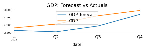
Figure 1. Forecast GDP and Actual GDP

We also use a set of indicators to estimate the forecast performance.

Table 4. Forecast Accuracy of GDP

5.2 Machine Learning Model

First, we put our data into five traditional models: Linear Regression; Support Vector Machine Regression; Random Forest Regression; Gradient Boosting Regression; K-Nearest Neighbors Regression. To compare the models, we will primarily use the default hyperparameters provided by Scikit-Learn. While these defaults generally yield decent performance, they should be optimized for better performance. At first, our goal is to establish a baseline performance for each model. Then, we will select some models for further optimization through hyperparameter tuning.

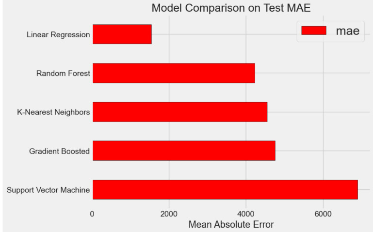
Figure 2. Model Comparison on Test MAE

According to the run, where results may vary slightly each time, the GBM performs the best, followed by the Random Forest models. Then, we will focus on optimizing the best-performing model through hyperparameter tuning.

We do hyperparameter tuning on gradient boosted model, linear regression model, and random forest model. In hyperparameter tunning, we use grid search to enumerate all the possible hyperparameter and compare their forecast result to find out the best hyperparameters.

We run the model on test set. In gradient boosted model, the performance of the model using default parameters is MAE= 4759.9017 while the performance of the optimized model after hyperparameter tuning is MAE =4474.0772.

The optimized model does exceed the baseline model by about 7% and has a great decline of running time (it's about 9.5 times faster).

To have a much direct sense of the performances, we draw the linear graph of real GDP values, the values from our final model prediction and the value from default model.

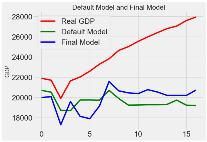
Figure 3. Gradient Boosting Model Prediction Comparison

Also, in Random Forest regression model, we run model on test set and the performance of the model using default parameters is MAE = 4262.0980 while the performance of the optimized model after hyperparameter tuning is MAE = 4202.1942.

The optimized model after hyperparameter tuning does exceed the baseline by about 1.5% and has a great decline of running time (it's about 1.56 times faster). To have a direct view of the difference, we plot the linear graph of real GDP values, the values from our final model prediction and the value from default model.

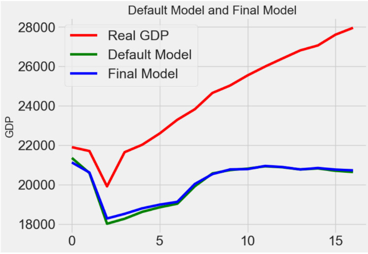
Figure 4. Random Forest Regression Model Prediction Comparison

In random Linear regression model, model after hyperparameter tunning performs the same as the default model. So, its final test set is still the default one: MAE = 1545.3309

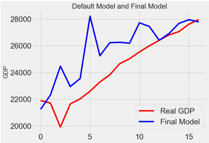
Figure 5. Linear Regression Model Prediction Comparison

After five traditional machine learning models, we also build RNN model to forecast GDP. The RNN (Recurrent Neural Network) Model is a type of neural network architecture specifically designed to deal with sequential data, especially the on with time order or logic order. This model is commonly used for ordinal or temporal data.

Unlike traditional machine learning models mentioned above, RNNs have connections that form cycles, allowing the network's output to depend not only on the current input but also on previous states. This structure makes RNNs well-suited for tasks involving time series data, natural language processing, and other sequential inputs.

We train the RNN model and use the testing set to evaluate it. Through the evaluation of the test set, the score of this model is MAE= 3537. Visualizing the difference between the predicted value and the actual value, we can find out that the gap between the forecast value and the actual value is enlarging.

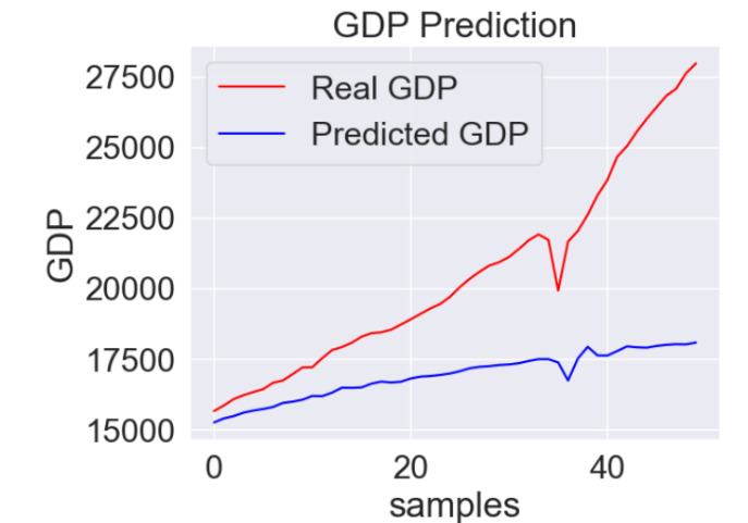
Figure 6. RNN Model Prediction Comparison

Compared with other traditional models like random forests, the predict value of RNN is not good. This may partly because traditional RNN models are always confronted with gradient vanishing or gradient explosion during training, which makes it difficult to learn long-term dependence effectively.

Thus, we will then introduce the LSTM model. LSTM is like an improved version of RNN model, which can solve the gradient vanishing or gradient explosion to a certain extent through the Gated Recurrent Unit, so that the network can be trained more stably.

We train the default LSTM model and then do hyperparameter tunning on it. The performance of default LSTM is MAE=11567.437, while the final model’s performance is MAE= 1036.531. The optimized model after hyperparameter tuning does exceed the baseline by about 11159.75%, which is a significant improvement in prediction. Visualizing the performance and the difference, we will draw the linear graph of real GDP, the predicted values from our final model and the predict value from default model.

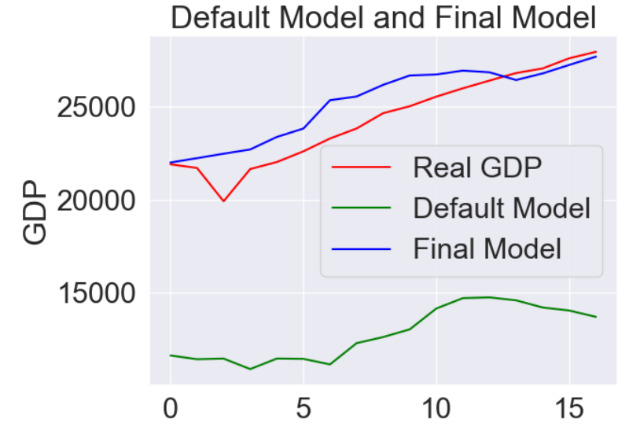
Figure 7. LSTM Model Prediction Comparison

After using several models to predict the US GDP, we have gotten the mean absolute mean of each model. As the chart below, LSTM model have the best performance on prediction. Thus, practically, the LSTM model seems to be the best choice.

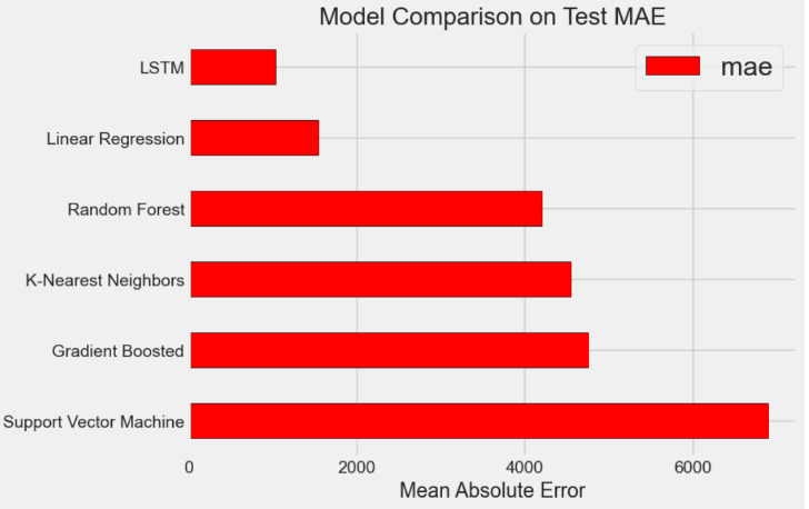
Figure 8. Model Comparison on Test MAE

Hence, LSTM model is the best choice. And we will continue Italy's GDP prediction using LSTM model.

6 Predictive Model of Italy

We will then use the LSTM model to forecast the Italy’s GDP. The input dataset has the following 12 quarterly time series:

GDP: Gross Domestic Product, Millions of Dollars, Quarterly, Seasonally Adjusted Annual Rate, from CEIC

unemploy: Infra-Annual Labor Statistics: Monthly Unemployment Rate Total: 15 Years or over for Italy, Percent, Quarterly, Seasonally Adjusted, from FRED

CPI: Consumer Price Index: All Items: Total for Italy, Growth rate previous period, Quarterly, Not Seasonally Adjusted, from FRED

PPI: Excl Construction, Index 2021=100, Quarterly, from Italian National Institute of Statistics

HOUSING: Residential Property Prices for Italy, Index Q1 1980=100, Quarterly, Not Seasonally Adjusted, from FRED

POPULATION: Population, Thousands, Quarterly, Not Seasonally Adjusted, from FRED

SHAREPRICE: Financial Market: Share Prices for Italy, Index Q1 1980=100, Quarterly, Not Seasonally Adjusted, from FRED

TREASURY: Interest Rates, Government Securities, Government Bonds for Italy, Percent per Annum, Quarterly, Not Seasonally Adjusted, from FRED

NON-TREASURY: Bond Rate: Average for Stocks, Percent, Quarterly, from Bank of Italy

EXPO: International Merchandise Trade Statistics: Exports: Commodities for Italy, Euro, Quarterly, Seasonally Adjusted, from FRED

IMPO: International Merchandise Trade Statistics: Imports: Commodities for Italy, Euro, Quarterly, Seasonally Adjusted, from FRED

SAVING RATE: Personal Saving Rate, Percent, Quarterly, Seasonally Adjusted Annual Rate, Calculated by Gross/Net National Savings from CEIC, Gross/Net National Savings from IMF

Also, we will preprocess the dataset before training the model. We normalize all the features, then the dataset is transformed into supervised learning problem. After reshaping the data set into the required format, we train the LSTM model and do hyperparameter tunning on it as well.

The performance of default LSTM is MAE= 170275.269, while the final model’s performance is: MAE= 70226.833. The optimized model after hyperparameter tuning does exceed the baseline by about 242.47%, which is a significant improvement in prediction. Also, visualizing the performance and the difference, we draw the linear graph of true values on the test set, the predicted values from our final model and the predict value from default model.

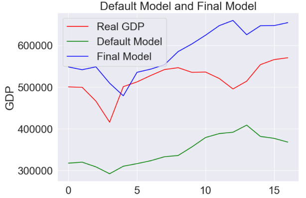
Figure 9. LSTM Model Prediction Comparison

Although the improvement of the final prediction of Italy’s GDP is not as good as the US’s one, we can say it’s a good prediction according to its MAE and trends in the graph. This may partly because the input data of Italy are not as concentrated as the US one and some of the input data are not counted by related departments, so we must use some similar indicators to replace them.

7 Limitation

According to the predictive result of US and Italy, the LSTM model performs best when forecasting the GDP compared to other algorithm like linear regression model and gradient boosted model. Also, hyperparameter tunning has a great improvement in the models’ performance. However, there is a huge gap between machine learning models traditional VAR models. In terms of numbers, they are still 2.6 times apart (400 vs 1036).

Machine learning is a kind of method that only focusing on the number’s features and ignoring the meaning behind these indicators. This is a huge limitation on using machine learning method to forecast the macroeconomic effects. Meanwhile, due to this feature, the accuracy of machine learning method hugely depends on the input data. If some input indicators are not collected or collected at a lower frequency like quarterly or annual which make this variable unavailable to the model, the performance of the model will decrease as our prediction of Italy’s GDP shows.

8 Conclusion

In conclusion, machine learning method have a good performance on forecasting the macroeconomic effects. And among all these machine learning models; LSTM models have the best performance. However, traditional VAR models outperform machine learning models in the accuracy. And the machine learning models’ performance rely on the input data heavily.

References

[1]. Eichenbaum, M. S., Rebelo, S., & Trabandt, M. (2020a). The macroeconomics of epidemics. NBER Working Papers 26882. National Bureau of Economic Research, Inc.
[2]. Eichenbaum, M. S., Rebelo, S., & Trabandt, M. (2020b). The macroeconomics of testing and quarantining. NBER Working Papers 27104. National Bureau of Economic Research, Inc.
[3]. Acemoglu, D., Chernozhukov, V., Werning, I., & Whinston, M. D. (2020). Optimal targeted lockdowns in a multi-group SIR model. NBER Working Papers 27102. National Bureau of Economic Research, Inc.
[4]. Baqaee, D. R., & Farhi, E. (2020). Supply and demand in disaggregated Keynesian economies with an application to the Covid-19 crisis. CEPR Discussion Papers 14743. C.E.P.R. Discussion Papers.
[5]. Baqaee, D., Farhi, E., Mina, M. J., & Stock, J. H. (2020). Reopening scenarios. NBER Working Papers 27244. National Bureau of Economic Research, Inc.
[6]. Favero, C. A., Ichino, A., & Rustichini, A. (2020). Restarting the economy while saving lives under Covid-19. CEPR Discussion Papers 14664. C.E.P.R. Discussion Papers.
[7]. Barro, R. J., Ursua, J. F., & Weng, J. (2020). The coronavirus and the great influenza pandemic: Lessons from the “Spanish flu” for the coronavirus’s potential effects on mortality and economic activity. NBER Working Papers 26866. National Bureau of Economic Research, Inc.
[8]. Barro, R. J. (2020). Non-pharmaceutical interventions and mortality in U.S. cities during the great influenza pandemic, 1918-1919. NBER Working Papers 27049. National Bureau of Economic Research, Inc.
[9]. Velde, F. (2020). What happened to the US economy during the 1918 influenza pandemic? A view through high-frequency data. Federal Reserve Bank of Chicago Working Paper No. 2020-11.
[10]. Baker, S. R., Bloom, N., Davis, S. J., & Terry, S. J. (2020). Covid-induced economic uncertainty (No. w26983). National Bureau of Economic Research.
[11]. Chetty, R., Friedman, J. N., & Stepner, M. (2024). The economic impacts of COVID-19: Evidence from a new public database built using private sector data. The Quarterly Journal of Economics, 139(2), 829-889.
[12]. Ludvigson, S. C., Ma, S., & Ng, S. (2020). COVID-19 and the macroeconomic effects of costly disasters (No. w26987). National Bureau of Economic Research.
[13]. Primiceri, G. E., & Tambalotti, A. (2020). Macroeconomic forecasting in the time of COVID-19. Manuscript, Northwestern University, 1-23.
Cite this article
Wei,Y. (2024). Using Big Data to Forecast Macroeconomic Effect during the COVID. Journal of Fintech and Business Analysis,1,45-55.
Data availability
The datasets used and/or analyzed during the current study will be available from the authors upon reasonable request.
Disclaimer/Publisher's Note
The statements, opinions and data contained in all publications are solely those of the individual author(s) and contributor(s) and not of EWA Publishing and/or the editor(s). EWA Publishing and/or the editor(s) disclaim responsibility for any injury to people or property resulting from any ideas, methods, instructions or products referred to in the content.
About volume
Journal:Journal of Fintech and Business Analysis
© 2024 by the author(s). Licensee EWA Publishing, Oxford, UK. This article is an open access article distributed under the terms and
conditions of the Creative Commons Attribution (CC BY) license. Authors who
publish this series agree to the following terms:
1. Authors retain copyright and grant the series right of first publication with the work simultaneously licensed under a Creative Commons
Attribution License that allows others to share the work with an acknowledgment of the work's authorship and initial publication in this
series.
2. Authors are able to enter into separate, additional contractual arrangements for the non-exclusive distribution of the series's published
version of the work (e.g., post it to an institutional repository or publish it in a book), with an acknowledgment of its initial
publication in this series.
3. Authors are permitted and encouraged to post their work online (e.g., in institutional repositories or on their website) prior to and
during the submission process, as it can lead to productive exchanges, as well as earlier and greater citation of published work (See
Open access policy for details).