1.Introduction

In light of the volatile nature of financial markets, it is required institutional investors keeps seeking for strategy to predict the performance of stock and select stock to trade dynamically. [1] examined several global economic factors and tried to use them to explain the volatility of stock price, after using regression method it found four important indicators which can explain large percentage of the variation in the volatility. While [3] introduced an approach to understanding investor sentiment and technological advancements. The book [6] saw the potential in the recent ’Data Science’ technologies and leveraged them to improve the performance of forecasting in economic and financial environments. And there are also other ways to predict stock prices, such as viewing it as a state of a Markov process [11] which is not considered in our paper.

Our study is inspired by the paper, “A Practical Machine Learning Approach for Dynamic Stock Recommendation,” [8] which utilizes machine learning methods to dynamically select and trade stocks from the S&P 500, also widely used in other papers such as [5]. Based on this foundation, our project expands the analysis by not only focusing on predictive modeling but also exploring the relationships between various market indicators such as opening and closing prices. In this paper, given lots of stock variables we conduct a thorough investigation into the correlations between opening and closing stock prices and also incorporate a rigorous hypothesis testing to validate our assumption. After that we define the daily return on each stock as the measure of the “potential” of a stock. Then we propose a comprehensive approach involving several regression models including Generalized Linear Regression, Gradient Boosting [7], and Random Forest [2], to forecast the return. Additionally, we use cross-validation to validate the models’ predictive capabilities.

This paper seeks to contribute significantly to the existing knowledge by providing empirical insights into the relationship of open-close price and other financial indicators. Through rigorous statistical analysis and advanced machine learning techniques, we generate several robust tools and methodologies that can guide in institutional investors in making daily decisions in the stock market. Our ultimate goal is to enhance the predictability of stock returns, then aiding in the development of more effective trading strategies which also required to leverage historical data to forecast future market behavior.

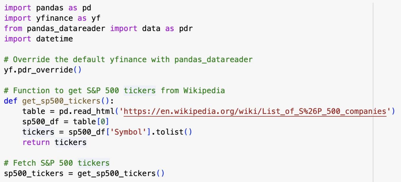
Figure 1. yfinance

2.Data

2.1.Data Sources

To ensure our data sample is comprehensive and unbiased, we decide to investigate the stock information for the S&P 500 component stocks, which cover approximately 80 percent of the American equity market by capitalization (S&P Global, n.d.). As suggested by Krauss and Stu¨binger [10], “This highly liquid subset of the stock market serves as a true acid test for any trading strategy.” To compile a comprehensive list of S&P 500 tickers, we utilized a function that programmatically fetched the data from Wikipedia’s ’List of S&P 500 companies’ page. This function employed the pandas library to read the HTML table on the page and extract the ticker symbols, ensuring an up-to-date repository of components for analysis.

To guarantee data accuracy and consistency, we utilized Python’s yfinance module to retrieve financial data from Yahoo Finance. We configured a loop using yfinance to fetch daily stock data for each stock listed on the S&P 500 over the past year (365 days) from our data collection date of April 22nd, 2024. In addition to the basic OHLC price information, which are built-in features of yfinance, we also collected additional data such as “Market Cap”, “Sector”, “PE Ratio”, “Revenue”, and “EPS”. These features provide a more detailed perspective of the market conditions and are critical in explaining the variability in our target variable, which is the expected return. In the following section, we will provide a comprehensive list of the features included in our dataset along with detailed descriptions to better understand their implications on our analysis.

2.2.Variable Interpretation

Our full dataframe consists of 125160 rows and 20 columns, capturing the daily dynamics of S&P 500 stocks. The temporal span of the data provides an invaluable longitudinal perspective, which is critical for assessing trends and performing time-series analysis within the volatile landscape of the stock market. Note that BRK.B and BF.B stocks are excluded from our dataset due to their different encoding in yfinance, which our data retrieval process could not capture. This strategic exclusion doesn’t compromise our dataset’s integrity, as we still have a wealth of stock information to work with. Each row of our dataset records a day’s data for an S&P 500 stock, and the columns record various features that provide a multi-dimensional view of each stock’s performance and underlying fundamentals.

Here’s a breakdown of the features in our dataset: Date: Represents the specific date for each data entry, ensuring chronological order which is crucial for time-series analysis. Stock Prices (OHLC): “Open,” “High,” “Low,” and “Close” prices provide insights into daily price volatility. We’re especially interested in the opening and closing prices, as these will help us calculate our main variable of interest. Volume: The number of shares traded in a day, indicative of the stock’s liquidity and investor interest. Dividends: Represents the return of value to shareholders and can signal company stability or profitability. Stock Splits: This factor adjusts for any splits in the stock that may artificially affect the stock price, ensuring data consistency over time. Ticker: The unique symbol representing each company in the stock market. Market Cap: The total market value of a company’s outstanding shares, reflecting its size and significance in the market. Sector: Categorizes companies into sectors, allowing for sector-specific analysis and comparison. PE Ratio: Price-to-Earnings ratio provides a valuation measure of a company’s current share price relative to its per-share earnings. Forward PE: An estimate of the future PE ratio, suggesting expectations of earnings growth or decline. Revenue: The total income generated by the company, a direct indication of its commercial activity. EPS: Earnings Per Share, a key indicator of profitability, determining the portion of a company’s profit allocated to each share of stock. PB Ratio: Price-to-Book ratio, compares a company’s market value to its book value, offering insights into how assets are valued in the market. Debt to Equity: This ratio assesses the financial leverage of a company, indicating how much of its operation is financed by debt compared to shareholders’ equity. Beta: A measure of a stock’s volatility in relation to the overall market, useful in assessing risk. Average Volume: The average number of shares traded over a specific period, smoothing out daily fluctuations in volume. Adj Close: The adjusted closing price accounts for any corporate actions like dividends or stock splits, providing a more accurate reflection of the stock’s value.

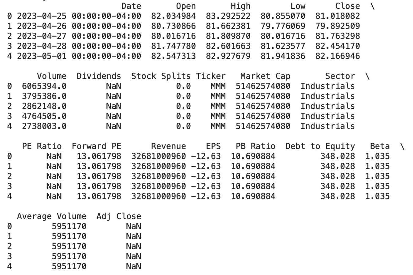
Figure 2: the vairables

These metrics play pivotal roles in our analytical framework. The financial indicators, such as the PE Ratio, Forward PE, EPS, and PB Ratio, allow us to evaluate each company’s financial health and market expectations. The market activity metrics, like Volume and Beta, give us an understanding of market behavior and risk. These features collectively impact the stock performance, we’ll build models in later sections to investigate how these features interact with each other and affect the returns.

2.3.Predictor Interpretation

How to use historical data to decide which stock I should trade today? It is the question we want to mainly solve. Then the following question is how to measure the “potential” of a stock. In our model, we define the daily return on each stock:

This return serves as a primary indicator of a stock’s daily performance, capturing the percentage change from the opening to the closing price. The simplicity of this measure belies its utility in revealing deeper market sentiments and trading dynamics.

The symbol and magnitude of the daily earnings not only reflect the immediate sentiment of the market, but also are key indicators of the future performance of the stock. Positive returns indicate bullish behavior by market participants, showing that at the end of the day investors are willing to pay more than the opening price. Negative returns, on the other hand, reveal a bearish trend, reflecting a decline in prices due to sales pressure or negative news. By paying close attention to these daily fluctuations, investors can capture market trends and key factors affecting the performance of individual stocks, leading to more accurate market forecasts.

The absolute value of daily returns as a measure of volatility provides important clues about the stability of a stock. A highly volatile stock that shows a large daily change in returns usually means greater investment risk but also indicates a higher return potential. This volatility information is an important part of building predictive models that allow analysts to assess the future movement of a particular stock or industry.

In addition, analyzing historical data on daily returns can significantly enhance the power of forecasting models. For example, time series analysis and machine learning techniques can use this data to predict price trends, providing a scientific basis for trading decisions. With these advanced analytical methods, investors can identify possible buying or selling times, especially when seeking quick returns through momentum trading strategies.

Combining daily earnings with other financial metrics, such as trading volume, price-to-earnings ratio and market cap, can further enhance the depth and accuracy of the analysis. High daily returns accompanied by high trading volume may indicate broad market agreement on the stock, while low trading volume with equal returns may mean a weaker market consensus, and this analysis allows investors to assess market dynamics more fully.

Therefore, daily earnings are a key tool for understanding and predicting stock performance, not only revealing the daily fluctuations of stock prices, but also providing an important basis for assessing market sentiment, investment risk, and future trends. With these insights, investors can make more scientific and strategic trading decisions and optimize the performance of their portfolios.

This kind of analysis emphasizes the importance of dealing with complex variables in stock trading, and the careful observation and interpretation of daily returns is the cornerstone of predicting and responding to market movements.

3.Data Preprocessing

3.1.Missing Data

To ensure the robustness of our analysis, we first performed calculations on the percentage of missing data in each column. By knowing how the missing values are distributed, we can then determine the best way to address each of these columns without compromising the integrity of our data. This is fundamental to our subsequent analysis, as the manner in which we handle missing data can significantly influence the results of our statistical modeling. For the columns “Dividends” and “Adj Close” which have too many missing values (> 90%), we decided to drop these columns since the available information in these columns would not suffice for an unbiased examination. For the column “Sector” that only has about 0.01 percent of missing values, we filtered the data frame to find the exact rows where the “Sector” value is NaN, and we figured out that only one stock with the symbol “GEV” has missing “Sector” information. Hence, we decided to drop this particular stock considering the vast amount of stock data left. For all other columns, since they are numerical variables and have relatively low amount of missing values, we employed the method of replacing the missing values with the respective column mean to preserve the original distribution of data. This treatment is based on Raymond’s findings that drawbacks mean imputation are negligible when less than 10% of the data is missing [13].

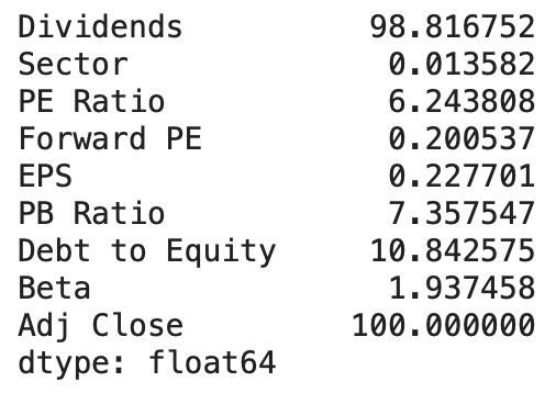
Figure 3. missing data

3.2.Check Data Normality

We generate QQ-plot for ’Open’ prices of stocks (same to ’Close’ prices of stock because of the small fluctuation per day). The QQ-plot for the ’Open’ prices exhibits a strong deviation from the red line, especially for higher quantiles. This is indicative of a skewed distribution, which is a common characteristic for financial data like stock prices. This plot tells us that large stock price movements are more common than what would be expected if the data were normally distributed. This could be the result of market volatility or other economic factors that create large swings in stock prices. The log transformation is a common technique used when dealing with data that has a multiplicative relationship, such as stock prices. After the log transformation, the QQ-plot for the log-transformed data shows that the points largely follow the red line, which indicates that the log-transformed data are approximately normally distributed. But we should notice that there are still some deviations from normality at both ends of the distribution, with the actual data being lighter in the tails than expected under a normal distribution.

Figure 4. Caption for both images

4.Hypothesis Test

In the previous section, we established that the distributions of both log open and log close prices are approximately normal. Given this, one might initially hypothesize that ’Log Return’, derived from these prices, would also follow a normal distribution.

However, the results from QQ-plots for ’Return’ and ’Log Return’ reveal both short-tailed distributions, contradicting the normality assumption. This discrepancy suggests that the returns do not exhibit the typical characteristics expected under a normal distribution. It is plausible that this could be attributed to the dependencies and interactions between these variables during the trading day, which has been extensively explored in the literatures, such as in Rebonato’s study on market volatility [14]. This insight leads us to reconsider the assumptions about the distributional properties of financial returns, taking into account the complex dynamics highlighted by previous research.

(a) Caption for image 1 (b) Caption for image 2

Figure 5. Caption for both images

To test the dependency between the ’Open’ and ’Close’ prices of stocks using pairwise correlation, we want to calculate the Pearson correlation coefficient ρ for these two variables, which is

where x_i and y_i are the values of two variables ’open’ and ’close’, ¯x and ¯y are the means of two variables ’open’ and ’close’. Null Hypothesis (H₀): There is no linear correlation between the ’Open’ and ’Close’ prices of stocks. Mathematically, this is represented as ρ = 0. Alternative Hypothesis (H₁): There is a significant linear correlation between the ’Open’ and ’Close’ prices of stocks. This is represented as ρ ̸= 0. The significance level α is set at 0.05 for this test. The rejection rule is that if the p-value is less than or equal to the significance level α, we reject the null hypothesis. Conversely, if the p-value is greater than α, we do not reject the null hypothesis. In python, we use the scipy.stats.pearsonr function to calculate the Pearson correlation coefficient and its two-tailed p-value. The p-value associated with the observed correlation coefficient is 0.0 which indicates an extremely small value, essentially meaning the correlation is highly significant statistically. We reject the null hypothesis and conclude that there is a significant linear correlation between the ’open’ and ’close’ prices of stocks. The very high correlation coefficient of approximately 0.9999 indicates that the relationship is very strong and positive. The close price of a stock is almost perfectly predicted by its opening price. This is consistent with the expectation that, the opening and closing prices should be very similar because they reflect the same trading day’s market conditions and sentiments.

In summary, the highly significant correlation between a stock’s ’Open” and its “Close” prices reveal a strong linear relationship, suggesting that closing prices can be almost completely predicted from opening prices. This discovery has several key implications. First, it may indicate that the market is extremely efficient, with new information quickly digested by the market, resulting in minimal price movements between opening and closing. It also suggests that price movements are less important during the trading day than information available at the opening.

In addition, the results stimulate further investigation into whether this model is universally applicable across different industries and market conditions. For example, through a comparative analysis of bull versus bear markets, we can explore whether external market forces have a significant impact on this correlation. This kind of analysis not only contributes to a deeper understanding of market dynamics, but may also provide market participants with more precise forecasting tools.

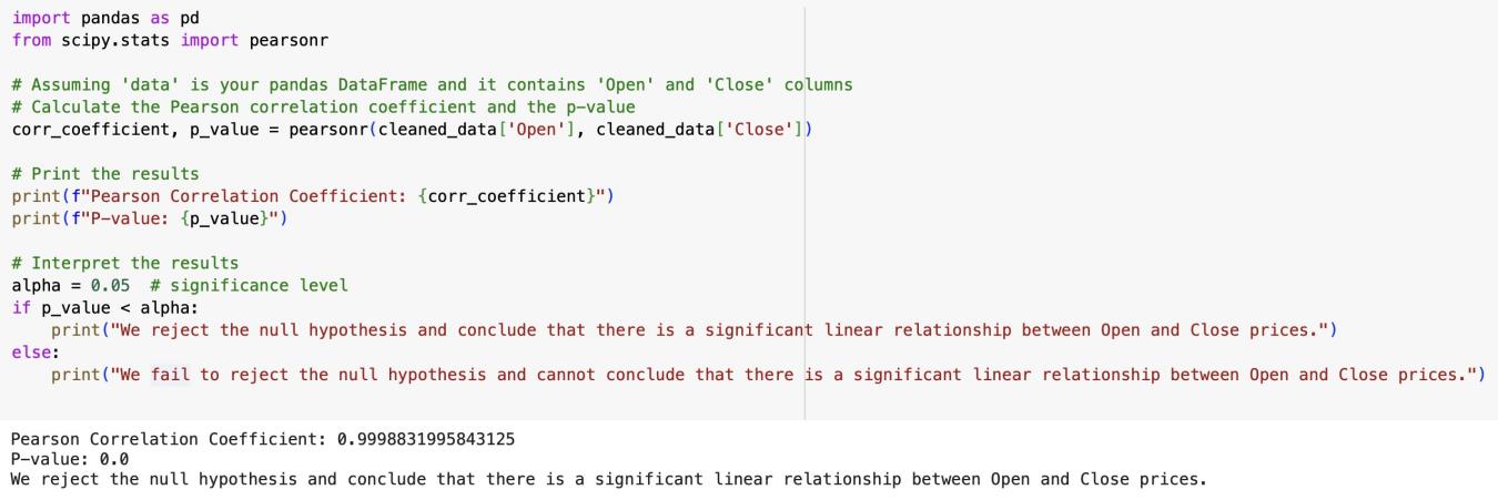
Figure 6. This frog was uploaded via the file-tree menu.

To substantiate our hypothesis, we generated a correlation matrix encompassing all relevant variables. This step allows us to quantitatively assess the dependencies among the variables, thereby testing the validity of our conclusions.

According to the correlation matrix, we can conclude the following results. High Correlation Between Open, High, Low, and Close Prices: These variables typically show a high degree of correlation in stock market data because they are directly related to the stock’s price for a given day. Volume and Average Volume: These are also highly correlated which is expected as they both measure the number of shares traded, though ’Volume’ is for a particular day and ’Average Volume’ might be averaged over a longer period. Market Cap and Revenue: There is a moderate correlation, which makes sense because companies with higher sales often have higher market valuations. PE Ratio, Forward PE, and PB Ratio: These variables are less correlated with price variables (Open, High, Low, Close) but are often more related to a company’s financial performance and market expectations. EPS (Earnings Per Share): This has a strong negative correlation with the PE Ratio, which can occur because the PE Ratio is calculated as the market value per share divided by the earnings per share. A higher EPS can lead to a lower PE if the stock price does not increase proportionally. Debt to Equity: Shows very little correlation with most other variables, suggesting that it moves quite independently of these factors in this particular dataset. Beta: Beta represents the volatility of a stock compared to the market. It shows low correlation with most of the financial metrics, implying that a stock’s volatility is not necessarily linked to its financials in a straightforward manner. Return1 and Return2: These could be daily returns or returns over different periods. If they represent consecutive periods (like day 1 and day 2), their correlation could be an indicator of momentum. If there’s no correlation, it might suggest that returns are random from one period to the next.

5.Model selection

5.1.Linear Regression

The first model selected for analysis is Linear Regression. Under this model, we first preprocess the numerical and non-numerical groups and exclude the datetime variable: ‘Date’. Then we convert categorical variables by using one-hot encoding and exclude non-numeric columns. After this, we update ‘features’ to include the new dummy variables and exclude the target variable ‘Return’. Then we start to split the train and test sets into ‘X train’, ‘X test’, ‘y train’ and ‘y test’. When finishing all these preparations, we start to build the regression model and predict on the testing set. Once the data is suitably prepared, the regression model is constructed and predictions are made on the test set. The model’s performance is assessed by calculating the Mean Squared Error (MSE), which yielded an estimated value of approximately 2.685e-25. This result, though not satisfactory, is consistent with expectations given the lack of data normalization, as discussed in Part 4. Consequently, it is concluded that Linear Regression is not an optimal fit for this dataset.

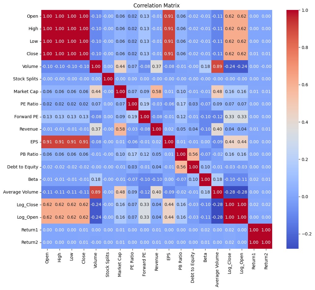
Figure 7. correlation matrix

5.2.Gradient Boosting

Given the unnormalized nature of our dataset, it is imperative to select models that are adept at handling such conditions. In this phase, we opt for Gradient Boosting to forecast our target variable, “Return”. We came up with this idea based on [4], ‘Besides avoiding tedious entitymatching, machine-learning models can form weakly-parametric estimators that are resilient to other imperfections in the data’. Initially, we import the ‘GradientBoostingRegressor’ from the ‘sklearn’ library and initialize the model, and initialize the Gradient Boosting Regressor model. Then we fit the model to the training data that we have already split above and predict on the testing set. Consistent with prior methodology, we use MSE to evaluate our results. The MSE for Gradient Boosting method is around 0.000979, which is a plausible outcome given the minimal range of our return data. Therefore, we can conclude that Gradient Boosting method has done a good job on predicting ‘Return’ and it is a suitable model for this dataset despite lack of normalization.

5.3.Random Forest

An alternative approach that we have explored is the Random Forest method. This method is considered because the inherent algorithm of random forest is not comparing the variable values, instead, it is splitting a sorted list that requires absolute value for branching [9]. The preparation of the data follows a similar protocol as previously described: identifying categorical columns, converting them using one-hot encoding, and ensuring that only numeric columns, excluding datetime columns, are retained for modeling. We define our features as all numeric columns except for our target variable, ’Return’, and subsequently divide the data into training and testing sets. Following data preparation, we initialize the Random Forest Regressor and fit the model to the training data.

To evaluate the model, we compute the MSE and get the result of around 0.00208, which is also a reasonable outcome since the range of our ‘Return’ is small. Thus, we conclude that the Random Forest method is another appropriate technique for predicting the ’Return’ variable in this dataset.

5.4.Bootstrap 500 times

Another approach we have tried is using Bootstrap for 500 times. We first define the number of bootstrap samples and prepare an array to store the bootstrap results. Then we use a for loop to perform the bootstrap method and compute overall results from the statistical result in the for loop. The average of the means calculated from each bootstrap sample is around 0.0174. This result serves as a robust estimate of the central tendency of the returns. The standard deviation of means is around 0.00415, which indicates that the bootstrap estimates of the mean return are relatively stable and do not vary widely across different samples. The other result we have got from the bootstrap method is that the mean of standard deviations is around 1.4378 indicating that, on average, the returns deviate from their mean by this amount. The last result we have got is standard deviation of standard deviations which is around 0.0092, indicating that the estimated variability of the returns is consistent across different bootstrap samples. Overall, the bootstrap results suggest that our estimate of average daily return is stable and consistent.

5.5.Generalized Linear Models

In addition, we also use the Generalized Linear Model to predict our target variable. We have come up with this idea by references [12] as it said, ‘Generalized linear models have greater power to identify model effects as statistically significant when the data are not normally distributed (Stroup xvii). Following the same steps of data preparation, we also add a constant to the features, which is often necessary for GLM. Then we define the dependent variable ‘Return’ and fit a generalized linear model. Here is the summary that we have got from this model: From this we can see each variable’s coefficient and the significant p values (¡ 0.05) indicates predictors are statistically significantly associated with the dependent variable. The Pseudo R-squ with value of 1.000 suggests a perfect goodness of fit. But there are potential concerns of overfitting, especially the model includes transformations of the dependent variable (like ‘Log open’).

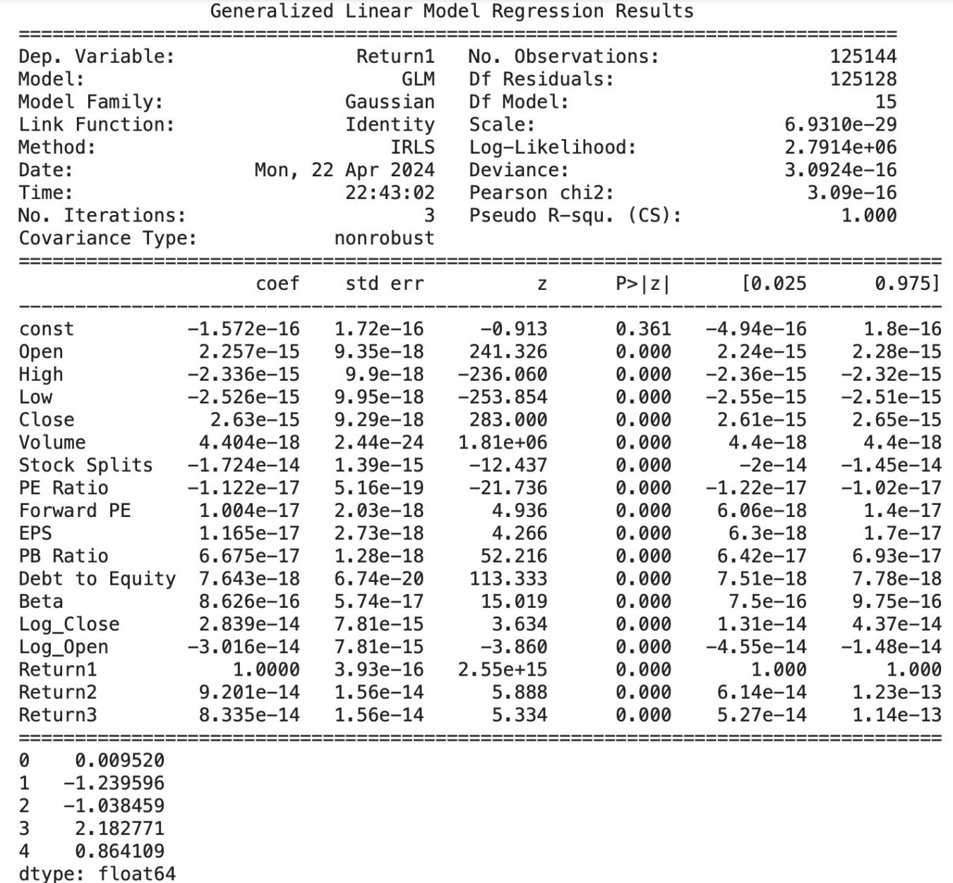
Figure 8. GLM results

6.K-fold Cross Validation

To validate the result, we have chosen K-folds Cross Validation and we choose k to be 12. Since only Gradient Boosting and Random Forest can be validate under this method, we have got the following result:

GradientBoosting − MeanMSE : 0.006780801632905623StddevMSE : 0.01951731864240686

RandomForest − MeanMSE : 0.008567523034390763StddevMSE : 0.025439335103457195

First of all, the Mean MSE from Gradient Boosting is around 0.00678. This relatively low mean MSE suggests that the Gradient Boosting model generally performs well in predicting the outcome across different subsets of the data. The other result, standard deviation of MSE with value around 0.01952 suggests some variability in the performance of the Gradient Boosting model across different folds. This means that the model could be sensitive to the specific subsets of data used for training. On the other hand, as for Random Forest, the Mean MSE is around 0.0085675. This Mean MSE is slightly higher compared to Gradient boosting, suggesting that it may not predict as accurately on average as Gradient boosting. While the Standard Deviation of MSE is around 0.02544 could imply that the model’s performance might vary more significantly with different training sets. This also suggests a potential overfitting or a model that is less robust to changes in the input data.

7.Conclusion

To achieve the goal of our research, we utilize the data both from yfinance and use pandas datareader to get the top 500 companies that we need. We also deal with the missing data, creating our variable ‘return’ and checking the normality of our data to prepare the data for our model. Under this process, we have found an interesting pattern of our data and use hypothesis testing to test our initial thoughts.

In conclusion, our comprehensive analysis has provided valuable insights into the dataset under this study. We have utilized five different models to predict our ‘Return’ variable and four of them have done a great job. The other one, Linear Regression, is not suitable for this project because our data is not normalized.

The bootstrap method revealed a stable estimate of the central tendency and dispersion of daily returns, indicating both the expected return and associated risk. The generalized linear model, with its near-perfect fit, suggested potential overfitting, but nonetheless highlighted key predictors influencing the returns. Cross-validation of the predictive models showed that gradient boosting outperformed the random forest in terms of mean squared error, suggesting a better fit for the data. However, the variability in the MSE across folds signaled the need for cautious interpretation and model validation.

Under this project, we shed light on the statistical properties and relationships within the data and also underscored the importance of rigorous validation techniques in modeling. As for more thoughts on this project, we could work on potential feature engineering, use time series to predict different stock’s daily performance, etc. Due to the limitation of our dataset, these are not achievable right now. However, with more information on the stock data, these thoughts are plausible and valuable to work on.

Authors’ Contributions

All the authors contributed equally to this work and should be considered as co-first authors.

References

[1]. Binder, J. J., & Merges, M. J. (2000). Stock market volatility and economic factors. Review of Quantitative Finance and Accounting. Available at SSRN: https://ssrn.com/abstract=265272 or http://dx.doi.org/10.2139/ssrn.265272.
[2]. Bin, O. A., Huang, S., Salameh, A. A., Khurram, H., & Fareed, M. (2022). Stock market forecasting using the random forest and deep neural network models before and during the COVID-19 period. Frontiers in Environmental Science, 10.
[3]. Baker, M., & Wurgler, J. (2007). Investor sentiment in the stock market. Journal of Economic Perspectives, 21(2), 129–152.
[4]. Cvetkov-Iliev, A., Allauzen, A., & Varoquaux, G. (2022). Analytics on nonnormalized data sources: More learning, rather than more cleaning. IEEE Access, 10, 42420–42431.
[5]. Caginalp, G., & Laurent, H. (1998). The predictive power of price patterns. Applied Mathematical Finance, 5, 181–206. Available at SSRN: https://ssrn.com/abstract=932984.
[6]. Consoli, S., Reforgiato Recupero, D., & Saisana, M. (2021). Data Science for Economics and Finance: Methodologies and Applications. Springer.
[7]. Davis, J., Devos, L., Reyners, S., & Schoutens, W. (2020). Gradient boosting for quantitative finance. Journal of Computational Finance, 24(4). Available at SSRN: https://ssrn.com/abstract=3829891.
[8]. Fang, Y., Liu, X.-Y., & Yang, H. (2019). Practical machine learning approach for stock trading strategies using alternative dataset. Available at SSRN: https://ssrn.com/abstract=3501239 or http://dx.doi.org/10.2139/ssrn.3501239.
[9]. KDnuggets. (2022). Random Forest Algorithm: Do We Need Normalization? https://www.kdnuggets.com/2022/07/random-forest-algorithm-need-normalization. [Online; accessed 25-April-2024].
[10]. Krauss, C., & Stübinger, J. (2015). Nonlinear dependence modeling with bivariate copulas: Statistical arbitrage pairs trading on the S&P 100. FAU Discussion Papers in Economics, 15/2015. Friedrich-Alexander University Erlangen-Nuremberg, Institute for Economics.
[11]. Nayanar, N. (2023). Interpreting institutional investment activity as a Markov process: A stock recommender. Intelligent Decision Technologies, 17(3), 1–13.
[12]. Ngo, T. H. D. (2016). Generalized linear models for non-normal data. https://support.sas.com/resources/papers/proceedings16/8380-2016.pdf. Accessed: 2024-04-25.
[13]. Raymond, M. R. (1986). Missing data in evaluation research. Evaluation & the Health Professions, 9(4), 395–420.
[14]. Rebonato, R. (2004). Volatility and Correlation: The Perfect Hedger and the Fox (2nd ed.). John Wiley & Sons.
Cite this article
Liu,Y.;Zhang,X.;Zhang,L. (2024). Daily Stock Selection. Journal of Fintech and Business Analysis,1,77-86.
Data availability
The datasets used and/or analyzed during the current study will be available from the authors upon reasonable request.
Disclaimer/Publisher's Note
The statements, opinions and data contained in all publications are solely those of the individual author(s) and contributor(s) and not of EWA Publishing and/or the editor(s). EWA Publishing and/or the editor(s) disclaim responsibility for any injury to people or property resulting from any ideas, methods, instructions or products referred to in the content.
About volume
Journal:Journal of Fintech and Business Analysis
© 2024 by the author(s). Licensee EWA Publishing, Oxford, UK. This article is an open access article distributed under the terms and
conditions of the Creative Commons Attribution (CC BY) license. Authors who
publish this series agree to the following terms:
1. Authors retain copyright and grant the series right of first publication with the work simultaneously licensed under a Creative Commons
Attribution License that allows others to share the work with an acknowledgment of the work's authorship and initial publication in this
series.
2. Authors are able to enter into separate, additional contractual arrangements for the non-exclusive distribution of the series's published
version of the work (e.g., post it to an institutional repository or publish it in a book), with an acknowledgment of its initial
publication in this series.
3. Authors are permitted and encouraged to post their work online (e.g., in institutional repositories or on their website) prior to and
during the submission process, as it can lead to productive exchanges, as well as earlier and greater citation of published work (See
Open access policy for details).