1. Introduction

In recent years, climate change and sustainable development issues have drawn widespread attention. Rapid industrial expansion and intensified human activities substantially increase greenhouse gas emissions, accelerating global warming and leading to more frequent extreme weather events. Many countries and regions, in response to climate change, have put forward the goals of carbon neutrality and net-zero emissions. As a means of reducing emissions, carbon emission trading has been applied globally and is regarded as crucial for the transition to a low-carbon economy. Currently, improving the precision of carbon price prediction, reducing corporate risks, and optimizing market functions in emission reductions have attracted growing academic and industrial attention.

Currently, academic discussions regarding carbon price forecasting mainly focus on three aspects: the carbon market price formation mechanism, influencing factors affecting carbon prices, and carbon price prediction models. Regarding the formation mechanisms of carbon market prices, prior studies have outlined the institutional frameworks of markets such as the EU and pilot carbon markets [1], analyzing their distinct price-setting characteristics [2]. For factors affecting carbon prices, research emphasizes identifying types and selecting crucial indicators, Zhao Lixiang et al. [3] summarized that the major factors influencing carbon prices, including policy dynamics, climate change, market environment, and energy prices. Chen Xin et al. [4] constructed a Bai-Perron structural break test from the perspective of supply and demand changes to observe the causes of drastic fluctuations in carbon prices. In terms of prediction approaches, the literature has proposed various methods, including econometric models, artificial intelligence algorithms, and hybrid techniques. Li et al. [5] employed empirical mode decomposition, GARCH models, and computable general equilibrium (CGE) models to predict China’s carbon prices based on historical data. Yao Yiqian et al. [6] developed a BP-LSTM hybrid neural network approach, demonstrating improved forecast accuracy.

Existing literature highlights that carbon trading prices are shaped by various market and non-market factors, but the challenge of accurately modeling these price dynamics remains unresolved. Traditional time series methods and machine learning approaches such as SVMs often fall short in capturing the complex nonlinear patterns observed in carbon price data. In contrast, Long Short-Term Memory (LSTM) networks, a refined class of recurrent neural networks, are designed to handle long-range dependencies in sequential data, making them highly suitable for time series forecasting tasks. However, the predictive accuracy of LSTM models is highly sensitive to hyperparameter selection, including the number of hidden units, learning rate, and time window size. Historically, these parameters have been set through manual tuning or grid search, processes that are often inefficient and heavily reliant on researcher expertise. To address this limitation, metaheuristic optimization algorithms have been increasingly applied to neural network hyperparameter tuning. Among them, the Particle Swarm Optimization (PSO) algorithm has attracted significant attention for its ability to efficiently explore large search spaces. Nevertheless, standard PSO can sometimes become trapped in local optima. The Hybrid Particle Swarm Optimization (HPSO) algorithm, which enhances the basic PSO by incorporating strategies such as elite and follower subgroups and cross-learning mechanisms, offers a promising solution. By integrating HPSO with LSTM, this study aims to develop a robust carbon price prediction model that overcomes the inefficiencies of manual hyperparameter tuning and achieves superior forecasting performance.

2. Research methodology

2.1. Long Short-Term Memory (LSTM) neural network

The Long Short-Term Memory (LSTM) is a special type of Recurrent Neural Network (RNN), which excels in learning long-term dependencies and is particularly suitable for time series prediction and classification. Its performance is influenced by hyperparameters such as the number of hidden units, the learning rate, and the prediction window. Optimizing these parameters can enhance the model's ability to capture long-term dependencies, its generalization performance, and the convergence speed. Therefore, in complex time series tasks, optimizing the hyperparameters of LSTM is crucial for improving the model's prediction ability and robustness. The basic unit structure of LSTM is shown in Fig 1. Each unit structure is composed of four main elements: the input gate \( {i_{t}} \) , the forget gate \( {f_{t}} \) , the output gate \( {o_{t}} \) , and the cell state \( {C_{t}} \) .

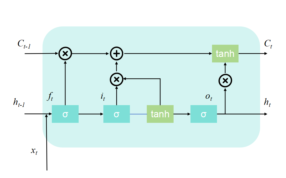
Figure 1: The basic unit structure of LSTM

2.2. Hybrid Particle Swarm Optimization (HPSO) algorithm

The HPSO algorithm divides the population into an elite subgroup and a follower subgroup, which are respectively responsible for different search tasks. The elite subgroup enhances its global search ability through a cross-learning strategy, while the follower subgroup improves its local search ability through a random learning strategy. The overview of the population learning strategy is as follows:

(1) Cross-learning strategy

In the HPSO algorithm, particles can reach the optimal state in each dimension. For the elite population, a horizontal crossover operator is designed to perform crossovers in the same dimension among the historical best positions of different particles, so as to enhance information sharing and improve diversity and global search ability. A vertical crossover operator is designed to avoid local optimality and perform crossovers between different dimensions of a single particle. In this paper, the velocity update formula is consistent with the traditional PSO velocity update strategy. The selection of the horizontal and vertical crossover operators in the position update formula depends on the value of rand and the crossover probability \( {p_{c}} \) . As shown in Equation (1), \( {r_{1}} \) , \( {r_{2}} \) and rand are random numbers uniformly distributed in the interval [0,1], \( j \) represents the index of another randomly selected particle, \( d≠{d_{1}} \) represents the feature dimension of the particle, and \( {d_{1}} \) is the other feature dimension of the particle randomly selected.

\( \begin{cases} \begin{array}{c} x_{id}^{t+1}={r_{1}}p_{id}^{t}+(1-{r_{1}})p_{jd}^{t}+c(p_{id}^{t}-p_{jd}^{t}), rand≤{p_{c}} \\ x_{id}^{t+1}={r_{2}}p_{id}^{t}+(1-{r_{2}})p_{i{d_{1}}}^{t}, rand \gt {p_{c}} \end{array} \end{cases} \) (1)

(2) Random learning strategy

In the follower subgroup, particles are sorted according to their fitness values, with the ones with poorer fitness at the rear. To guide the particles with poor fitness to search for a better solution space, a random learning strategy is designed. Assume that after sorting, particle \( {x_{i}} \) randomly selects a particle \( {x_{k}} \) from the first \( i-1 \) particles as the learning object, and performs a crossover operation as shown in Equation (2) to generate a velocity vector. Using this velocity vector, the particles with poor fitness can learn from the experience of the better - performing particles and explore their solution space, thus obtaining a new position. As shown in Equation (3), \( {r_{1}} \) , \( {r_{2}} \) , and rand are random numbers uniformly distributed in the interval [0,1] and \( {p_{m}} \) is the mutation probability.

\( v_{id}^{t+1}=ωv_{id}^{t}+{c_{1}}{r_{1}}({r_{2}}p_{id}^{t}+(1-{r_{2}})p_{kd}^{t}-x_{id}^{t}) \) (2)

\( \begin{cases} \begin{array}{c} x_{id}^{t+1}=p_{id}^{t}+{c_{2}}{r_{2}}(p_{gd}^{t}-p_{id}^{t}), rand≤{p_{m}} \\ x_{id}^{t+1}=x_{id}^{t}+v_{id}^{t}, rand \gt {p_{m}} \end{array} \end{cases} \) (3)

3. Carbon price prediction model based on HPSO-LSTM

This study applies the HPSO algorithm to optimize key hyperparameters of the LSTM model—including time window size, hidden unit count, dropout probability, and learning rate—thereby reducing manual bias. To improve the algorithm’s efficiency, the HPSO design is modified by keeping the horizontal crossover operator in the cross-learning process while substituting the vertical crossover operator with the standard PSO position update method. This results in the development of an HPSO-LSTM-based carbon price forecasting model.

\( \begin{cases} \begin{array}{c} x_{id}^{t+1}={r_{1}}p_{id}^{t}+(1-{r_{1}})p_{jd}^{t}+c(p_{id}^{t}-p_{jd}^{t}), rand≤{p_{c}} \\ x_{id}^{t+1}=x_{id}^{t+1}+v_{id}^{t+1}, rand \gt {p_{c}} \end{array} \end{cases} \) (4)

The procedure for the HPSO-LSTM model is illustrated in Fig 2:

Step 1: Preprocess the experimental data, including historical carbon prices and relevant influencing variables; divide the dataset into training, validation, and test subsets.

Step 2: Define the time window, hidden layer units, dropout rate, and learning rate as optimization targets, and initialize the particle swarm parameters.

Step 3: For each particle, construct an LSTM model using its position as hyperparameters, train it on the training set, validate it, compute the mean squared error (MSE), and assign it as the particle’s fitness value.

Step 4: Rank particles based on fitness, identify each particle’s best historical position and the global best position, and split the population into elite and follower subgroups according to the predefined elite proportion.

Step 5: The elite group applies the cross-learning strategy to update velocity and position using the crossover probability and Equation (4); the follower group uses the random learning strategy, updating velocity and position via the mutation probability and Equations (2)-(3).

Step 6: Check termination criteria. If met, return the best hyperparameter set; if not, repeat from Step 3 until the stopping condition is fulfilled.

Step 7: Build a final LSTM model using the optimized hyperparameters, retrain it on the training set, generate predictions on the validation and test sets, and assess model performance.

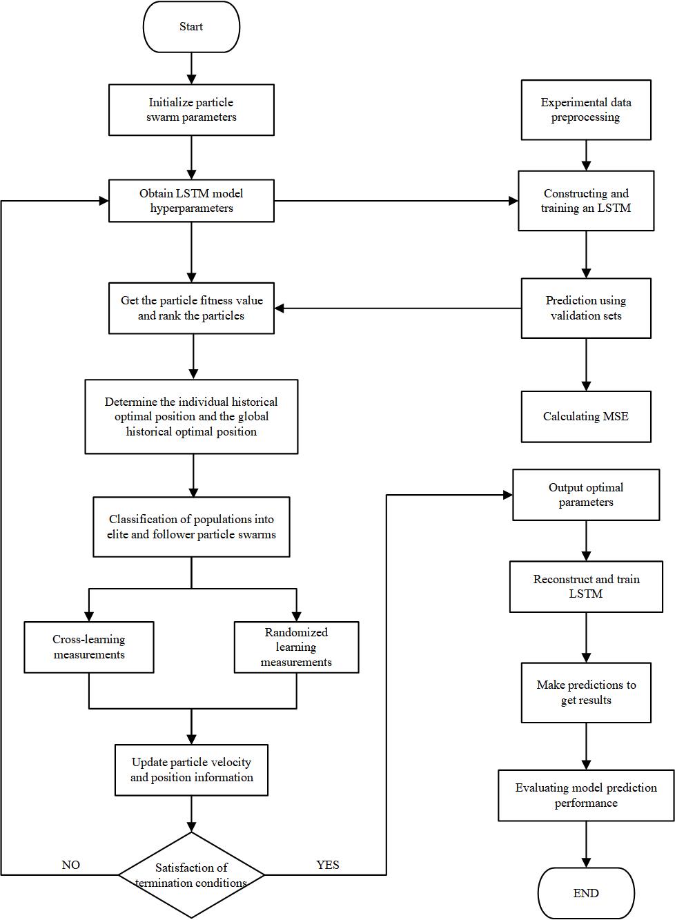
Figure 2: Algorithm flowchart of the HPSO-LSTM model

4. Empirical analysis

4.1. Data source and preprocessing

The dataset used in this study includes daily closing prices from China’s national carbon trading market, alongside variables such as the CSI 300 Index and the EU Emission Allowance (EUA) prices. The time span ranges from July 16, 2021, to June 7, 2024, totaling 701 observations. The CSI 300 Index serves as a proxy for China’s macroeconomic trends, while EUA prices represent international carbon market benchmarks. Energy market indicators include prices for coking coal, INE crude oil, and UK natural gas (IPE). Descriptive statistics of all variables are presented in Table 1.

Table 1: Descriptive statistical results of the data

4.2. Model parameter settings and evaluation indicators

The LSTM prediction model is composed of two hidden LSTM layers followed by a fully connected output layer. The HPSO algorithm is utilized to optimize four key hyperparameters: time window length, number of hidden units, dropout probability, and learning rate. Each of the four dimensions of the particle vector corresponds to one hyperparameter. Their respective ranges are set as [1, 30], [16, 256], [0, 0.5], and [0.001, 0.01], with maximum velocities configured to 2, 8, 0.01, and 0.001. The particle swarm includes 50 individuals and evolves over a maximum of 100 iterations. The inertia weight decreases linearly from 0.9 by 0.005 per generation. Learning factors, elite group ratio, crossover probability, and mutation rate are all initialized at 0.5. During optimization, each LSTM model is trained over 100 epochs using the Adam optimizer and MSE as the loss function. For comparative purposes, an MLP model with the same configuration is used as a benchmark.

To evaluate the prediction accuracy of the model, four commonly used evaluation indicators are introduced: Mean Absolute Error (MAE), Root Mean Squared Error (RMSE), Mean Absolute Percentage Error (MAPE), and \( {R^{2}} \) . MAE, RMSE, and MAPE are used to detect the deviation between the predicted values and the true values of the model, and \( {R^{2}} \) reflects the fitting degree of the model to the data. The closer \( {R^{2}} \) is to 1, the better the model fits the data.

4.3. Analysis of experimental results

Fifty percent of the samples in the dataset are used as the training set, 20% as the validation set, and 30% as the test set. In Experiment 1, only the historical carbon price data is used as the input for prediction. In Experiment 2, on this basis, the influences of multiple factors such as the macro environment, the international carbon market, and energy prices on the carbon price are further considered, and multiple variables are used for comprehensive prediction of the carbon price. The HPSO algorithm is respectively used to optimize the hyperparameters of the LSTM model for Experiment 1 and Experiment 2. The population evolution curves are shown in Fig 3(a) and 3(b), and the optimal hyperparameters of the finally obtained LSTM model are shown in Table 2. It can be seen from Figure 3(b) that in Experiment 2, a relatively good LSTM model has been obtained when initializing the population, resulting in the long-term stagnation of population evolution. With the increase of the mutual learning among particles in the elite subgroup and the follower subgroup, the population jumps out of the local optimum in the later stage and quickly converges to a better state. To a certain extent, this result shows that the adjusted HPSO algorithm has not lost its original strong global search ability and can effectively reduce the risk of falling into local optimum during the population evolution process.

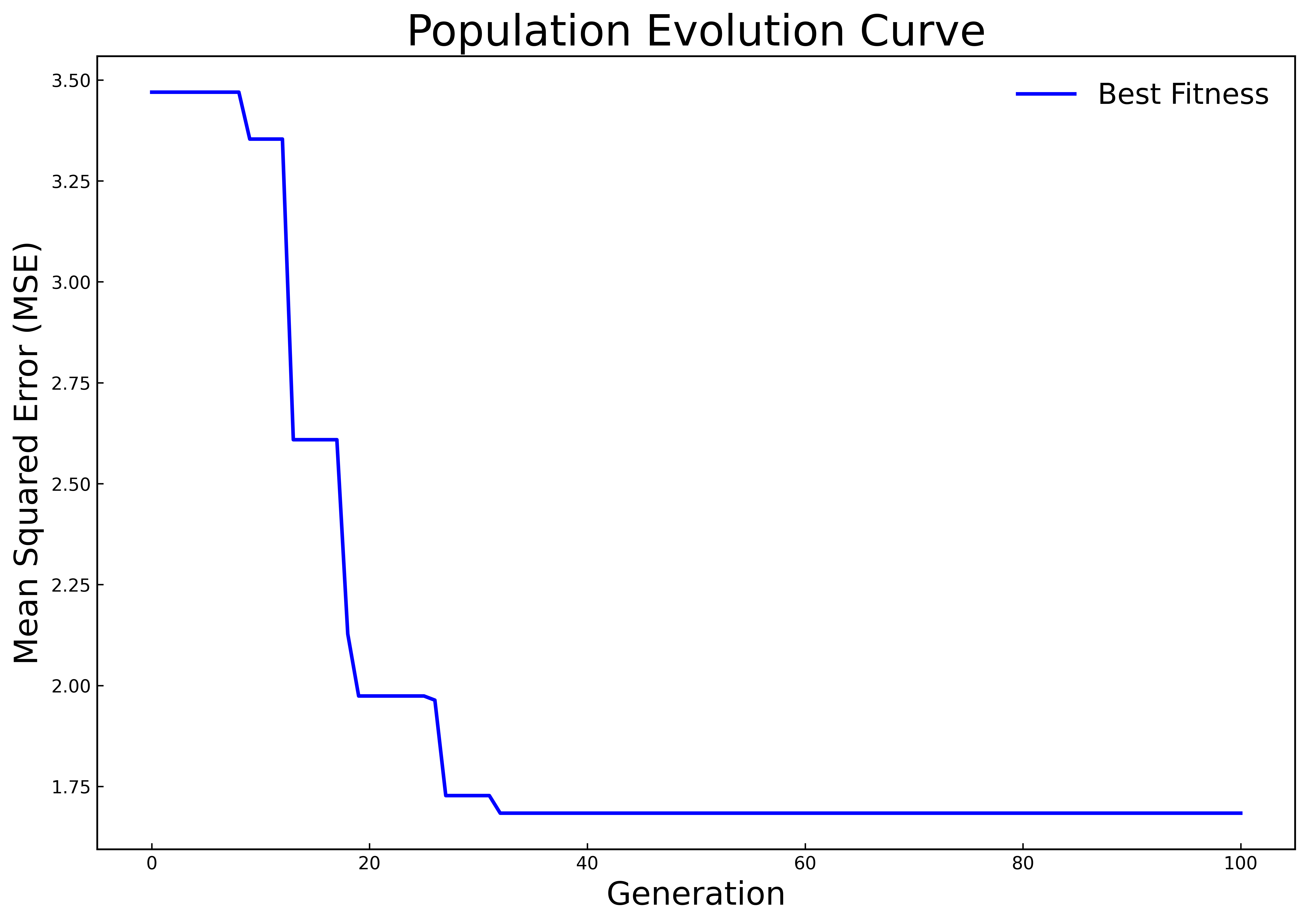
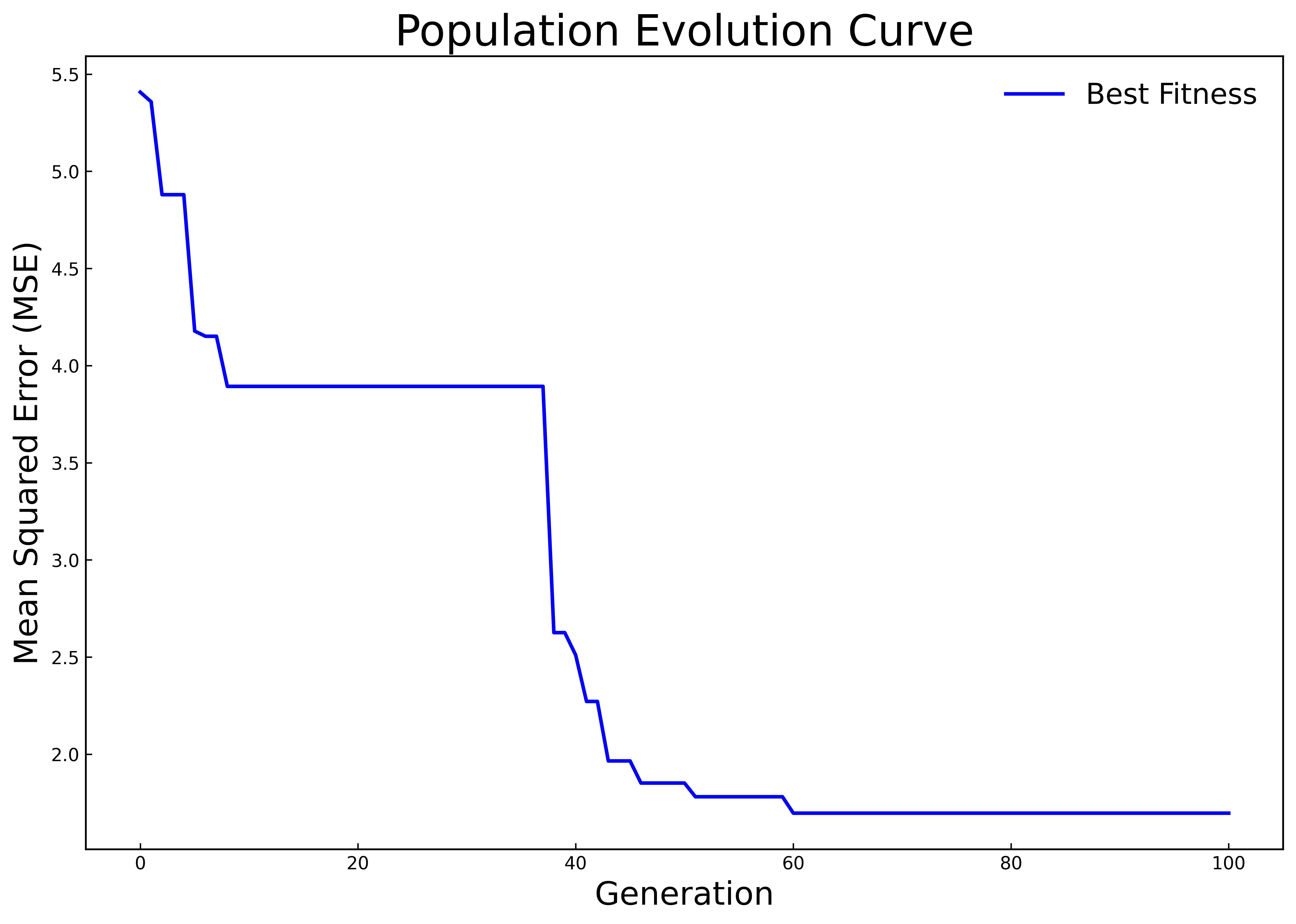
Table 2: The results of hyperparameter optimization of LSTM by HPSO

Based on the optimal hyperparameters, the LSTM models are reconstructed and trained respectively, and the number of iterations is changed to 200. The validation set and the test set are combined for prediction. The prediction results of the models in Experiment 1 and Experiment 2 are shown in Fig 4 and Fig 5, and the evaluation results of the model prediction performance are shown in Table 3. It can be seen that whether it is predicting with only the historical carbon price data as the input or conducting comprehensive prediction with multiple variables, the prediction model after optimizing the hyperparameters of the LSTM model by the HPSO algorithm has a better fitting effect and smaller prediction errors compared with the MLP model, and can predict the carbon price more accurately. In addition, it can be concluded from the experimental results that further incorporating the data of the influencing factors of the carbon price into the prediction model on the basis of the historical carbon price data can predict the future carbon price more accurately. In comparison to using historical carbon price data alone, prediction accuracy improved by 26.3%, 25.7%, and 25.6%, with goodness-of-fit increasing by 2.1%.

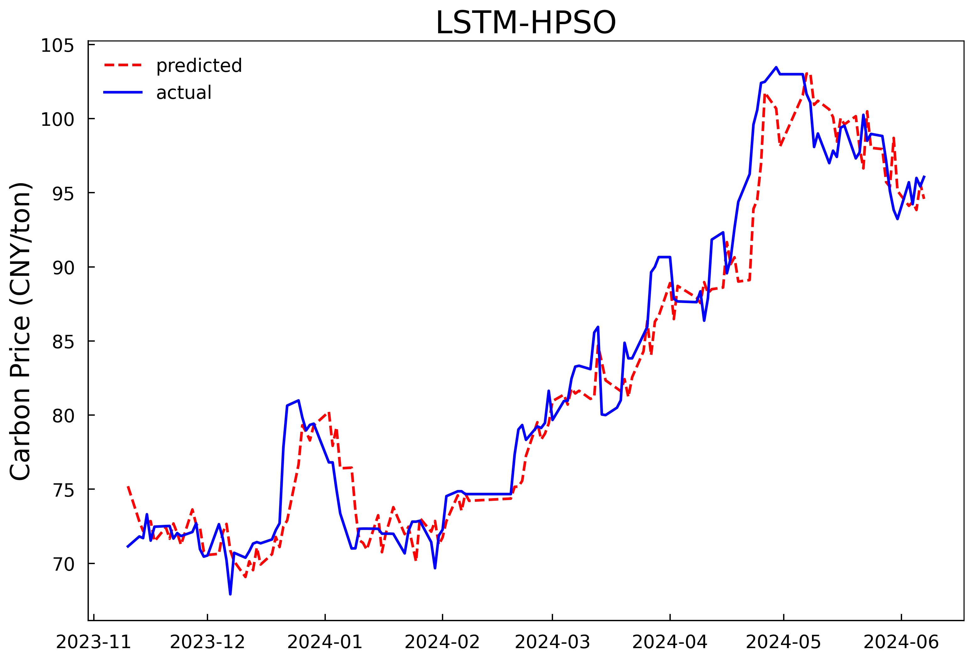
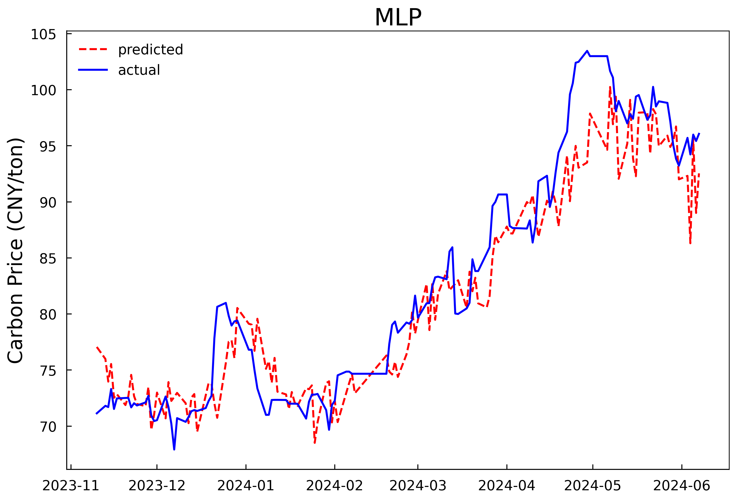
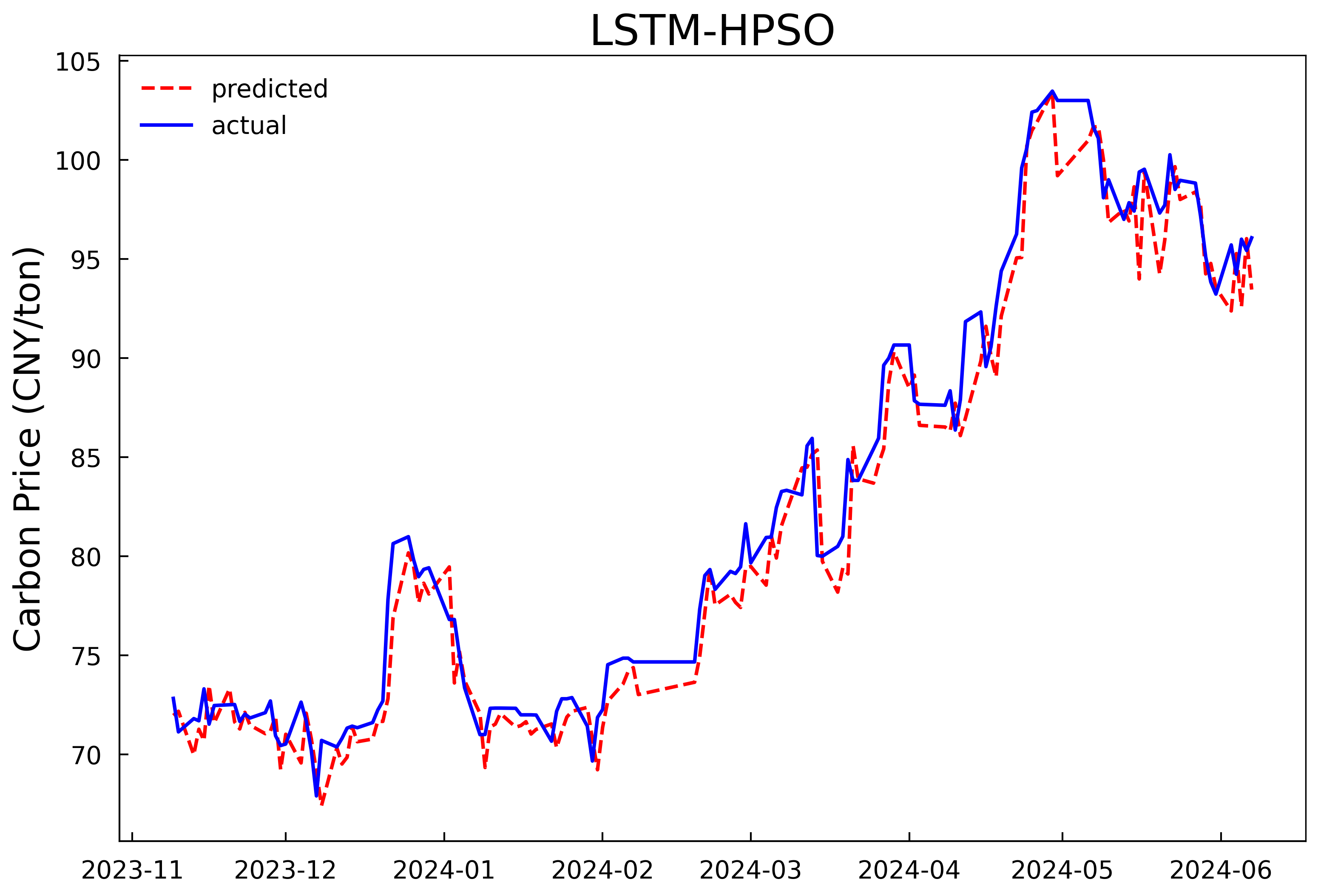
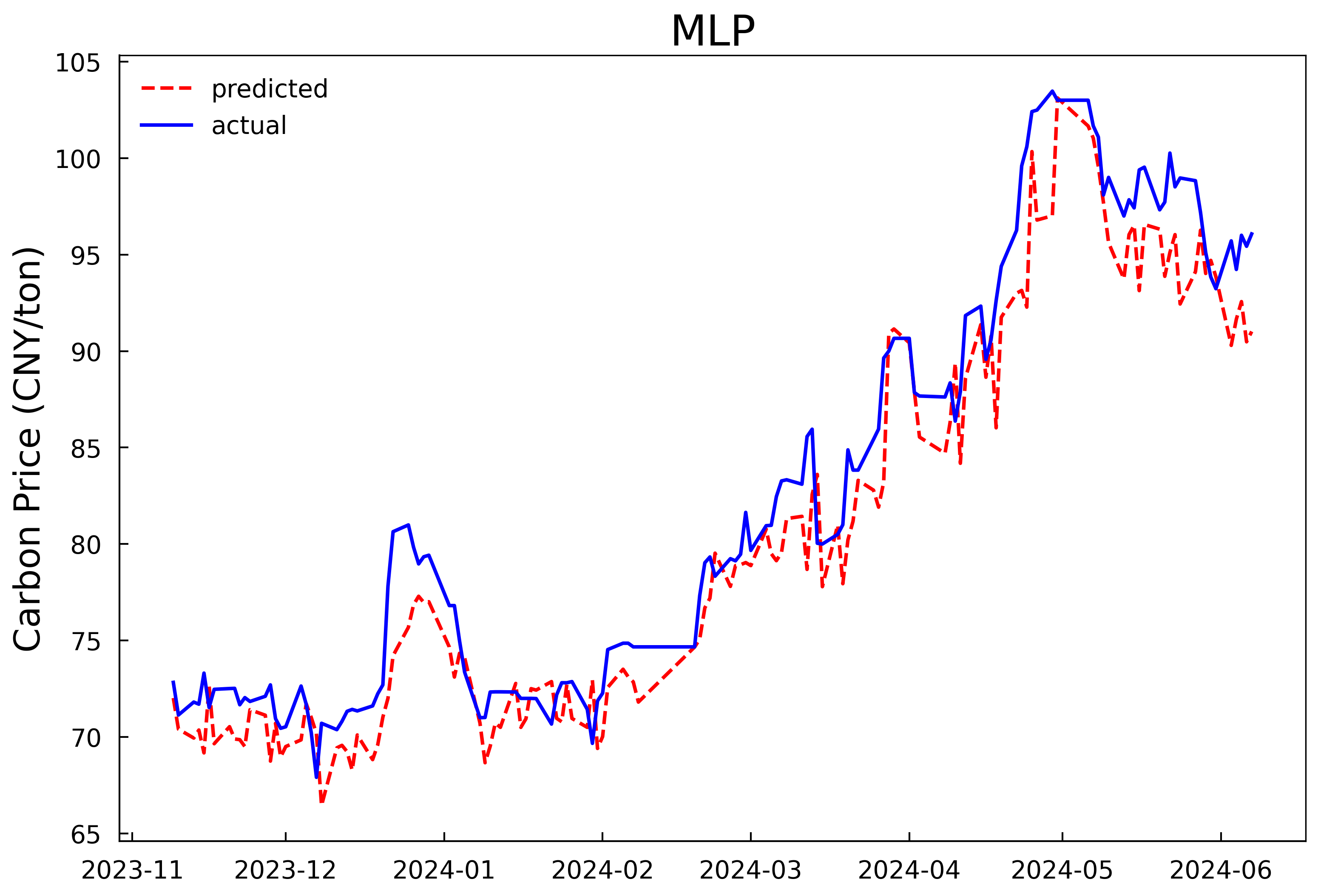
Table 3: Comparison of model prediction performance evaluation indicators

5. Conclusion

Aiming at the complex nonlinear carbon price prediction problem, this paper combines the hybrid particle swarm optimization algorithm and the LSTM neural network to construct a carbon price prediction model based on HPSO-LSTM. Then, a time series prediction of the national carbon price is carried out by only considering the historical carbon price data, as well as a comprehensive prediction with multiple variables by comprehensively considering the historical carbon price data, the macro environment, the international carbon market, and energy prices. The research results show that the HPSO algorithm has a strong global search ability and can be effectively used for the optimization of LSTM hyperparameters, thus avoiding the subjectivity of manually setting and adjusting hyperparameters. The optimized LSTM model has a high prediction accuracy and goodness of fit, and the prediction effect of the comprehensive prediction model with multiple variables is better than that of the time series prediction model. In the future, other factors such as text features and the degree of public attention can be considered for predicting the carbon price to further improve the prediction accuracy of the model.

References

[1]. Zhang, J. J., Wang, Z. X., & Lei, Y. W. (2020). The Enlightenment of the EU Carbon Market Experience to the Construction of China's Carbon Market. Price: Theory & Practice, (1), 32-36, 170.
[2]. Chen, Z. B., & Sun, Z. (2021). The Development Process of China's Emission Trading Scheme: From Pilots to a National Market. Environment and Sustainable Development, 46(2), 28-36.
[3]. Zhao, L. X., & Hu, C. (2016). Research on the Influencing Factors of China's Emission Trading Price: An Empirical Analysis Based on the Structural Equation Model. Price: Theory & Practice, (7), 101-104.
[4]. Chen, X., Liu, M., & Liu, Y. (2016). Driving Factors and Structural Breaks of Carbon Trading Prices: An Empirical Study Based on Seven Carbon Trading Pilots in China. On Economic Problems, (11), 29-35.
[5]. Li, W., & Lu, C. (2015). The Research on Setting a Unified Interval of Carbon Price Benchmark in the National Carbon Trading Market of China. Applied Energy, 155, 728-739.
[6]. Yao, Y. Q., Hong, R., & Liu, Q. Y. (2023). Research on Carbon Price Prediction Based on BP-LSTM Hybrid Neural Network. Environmental Science and Management, 48(9), 71-76.
Cite this article
Chen,D.;Shi,C. (2025). Carbon Trading Price Prediction Research Based on HPSO-LSTM. Applied and Computational Engineering,163,7-14.
Data availability
The datasets used and/or analyzed during the current study will be available from the authors upon reasonable request.
Disclaimer/Publisher's Note
The statements, opinions and data contained in all publications are solely those of the individual author(s) and contributor(s) and not of EWA Publishing and/or the editor(s). EWA Publishing and/or the editor(s) disclaim responsibility for any injury to people or property resulting from any ideas, methods, instructions or products referred to in the content.
About volume
Volume title: Proceedings of the 3rd International Conference on Software Engineering and Machine Learning
© 2024 by the author(s). Licensee EWA Publishing, Oxford, UK. This article is an open access article distributed under the terms and
conditions of the Creative Commons Attribution (CC BY) license. Authors who
publish this series agree to the following terms:
1. Authors retain copyright and grant the series right of first publication with the work simultaneously licensed under a Creative Commons
Attribution License that allows others to share the work with an acknowledgment of the work's authorship and initial publication in this
series.
2. Authors are able to enter into separate, additional contractual arrangements for the non-exclusive distribution of the series's published
version of the work (e.g., post it to an institutional repository or publish it in a book), with an acknowledgment of its initial
publication in this series.
3. Authors are permitted and encouraged to post their work online (e.g., in institutional repositories or on their website) prior to and
during the submission process, as it can lead to productive exchanges, as well as earlier and greater citation of published work (See
Open access policy for details).