1.Introduction

The architecture of the convolutional neural network (CNN) has been evolved for many years. In this process, there are lots of variant structures published from different opinions. Since the impressive architecture of AlexNet, the accuracy of ImageNet classification work improves significantly in 2012 [1]. In the following years, VGG, GoogLeNet, ResNet, Inception v3, SqueezeNet appear successively in the field of CNN [2-6]. With the contribution of those originator, descendants could reach another higher level of efficiency and accuracy. The development of architectures on CNN could generally describe like an oak. Its sturdy trunk is the working principle and central idea of CNN. Branches are the variants of novel architectures. Some of the designers who update the architecture also could solve the leftover problem on the previous layout by innovating the novel strategy or mixing the advantage from various architectures.

At early stage, the outcome from the experiment of VGG model reminds scientists that the depth (number of layers in the structure) is beneficial for the classification accuracy [2]. In other words, the accuracy may increase when models increase the number of layers. After the spread of that statement worldwide, the influx of institutions starts researching the effect of “deeper layers” architectures. Surprisingly, the result from a great number of experiments reflects a doubt: Adding more layers veritably represents the better networks? One of the successful studies about this topic revisit the reason of this phenomena and propose a fresh idea to solve it. It is the new model named ResNet [4]. Due to the stacking of layers, the vanishing gradients problem (the gradient descent never converges to the optimal) and the exploding gradients problem (the gradient becomes bigger and bigger) reversely increase the error rate. Thus, ResNet introduces a deep residual learning framework to smooth out the difficulties for setting up a deeper model.

Beside the promotion on enlargement of model depth, there is another researching school on CNN model. The aspiration is to construct a lightweight architecture. It aims to reduce the computational cost and return relatively reliable output. This type of research intelligently ingratiates the era of mobile internet. For example, CNN models have native advantage to deal with the work of vision [7]. With the limitation of storage space and power consumption, they are suitable when servicing to some applications on mobile devices, such as face recognition, beautification camera and autonomous driving. In other words, lightweight models provide the opportunity to apply the CNN technique on most mobile devices. In recent years, SqueezeNet, MobileNet, EfficientNet have already harvest some remarkable achievements, including the inclusive compression algorithm, different searching space and searching strategy [6-8].

From the regular model which expanding the number of nodes to catch accurate feature to the lightweight model that sacrificing the advantage of depth to satisfy the requirements of portability, it is simple to discover their common characteristics on the evolution. Every iteration of architectures is based on the flaw of previous models. With the birth of various techniques and strategies, this article illustrates some outstanding models in both branches as well as discussing why they can do better, thereby reflecting to its research trend and raising some guesses.

2.Benchmark Dataset

2.1.ImageNet

ImageNet is a large-scale ontology of images based on the WordNet hierarchy [9]. This dataset is one of the benchmarks in the field of image classification. During the ImageNet Large Scale Visual Recognition Challenge (ILSVRC), many participants use its labelled images to train and validate their models. Even though the ILSVRC ends in 2017, ImageNet still unremittingly services for a large amount of researching paper. Figure 1 shows the comparison of the usage among three popular datasets in different year, over thousands of experiments choose ImageNet as their dataset. Therefore, the reputation and reliability of ImageNet has proven by time.

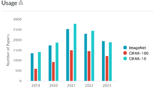
Figure 1. The usage of different dataset from 2019 to 2023 [10].

2.2.Evaluation Method

Controlling variables is fair and visualized method to measure the performance of models. During the analysis, every model can only be selected when ImageNet dataset ever participated in the experiment. Accuracy rate is one of the important indicators to evaluate the performance of models. The advanced model should have better percentage on accuracy. Besides, the number of parameters is another necessary factor. This number indicates the scale of models. For example, the expand of layers or channels increases the number of parameters. It intuitionistic reflects the consumption of resource, such as power, processor, memory capacity. Hence, Accuracy rate and the number of parameters support the argumentation from various nominated CNN models.

3.Models

3.1.ResNet

ResNet plays an important role in the development of CNN architectures. Deep residual learning framework is the core and revolutionary update in the ResNet structure. The metaphor of the new strategy is called ‘shortcut-connection’ (Figure 2) [4]. The shortcut is an identity mapping, which is the same as the input on starting layer. Another route is the residual mapping. It represents the improvement of the following layers. On the extreme case, the output at the end of shortcut connection has no modification compared to the input on starting layer, if the residual is easier to push to zero.

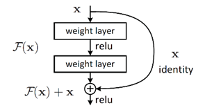
Figure 2. A block of residual learning [4].

The structure of residual learning brings the possibility to attach more layers. Results are shown in Table 1. When the depth of layer increases, error rate from plain network rises. On the contrary, ResNet relies on its skipping strategy, error rate remarkably decreases [4].

Table 1. Top-1 error on ImageNet validation.

3.1.1.ResNet-RS

ResNet-RS is one of enhanced version published in 2021. It not only inherits the benefit on the depth of layers from residual learning framework, but also finds that training and scaling strategies may matter more than architectural changes. From Figure 3, it could be observed that the top-1 ImageNet Accuracy has larger increase when improving with modern training methods than the increase of architectural changes [11].

The improvement of training strategies significantly refines the accuracy rate. Regularization such as dropout, label smoothing, stochastic depth, weight decay, data augmentation improves the generalization. For example, the method of dropout (CNN) is one common technique to predict the forward weight by the probability.

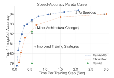
Figure 3. Blue dash line represents the top-1 accuracy of model ResNet-RS [11].

Throughout the experiment of ResNet-RS, it discovers that width, depth, and image resolution can highly affect the performance of models. If the epoch regime is long, depth scaling is better than width scaling. Conversely, width scaling outperforms depth scaling when epoch regime is shorter [11]. There is a verification based on three epoch regimes (Figure 4: Left-10 epochs / Middle-100 epochs / Right-350 epochs). Four different training image resolutions (128, 160, 224, 320) on training. The variance in the graph proves the appropriate scaling strategy depends on its training regime [11].

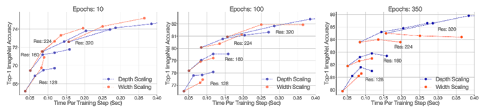
Figure 4. The comparison of depth scaling and width scaling on different epochs regime [11].

The second discovery on scaling strategy is ‘slow image resolution scaling’ [11]. The resolution gradually increases when model goes deeper. It truly speeds up as well as improves the accuracy of the model. In figure 5, ResNet-RS-152-192 (format: ResNet-RS-depth-image resolution) is one of the blue nodes. Comparing to ResNet-RS-152-256, the model with higher image resolution has better accuracy when both models have the same depth [11].

Figure 5. Comparison on Speed-Accuracy Pareto Curve between ResNets-RS and EfficientNet [11].

Even though the contribution on the progress of accuracy is not significant like the strategies talking above, it is another practicable way. In this case, ResNet-RS is the combination of modified ResNet-D and Squeeze-and-Excitation (SE). SE is a method to reweigh the feature map via a squeeze operation of global average pooling. Corresponding results are shown in Figure 6 [12].

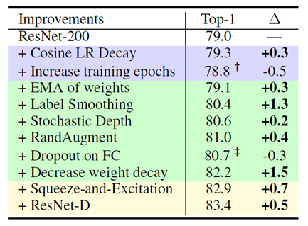
Figure 6. The list of improvements on ResNet-RS. Purple-training methods, Green-regularization methods, Yellow-architecture improvements [11].

3.1.2.Inception-ResNet

Inception-ResNet is on hybrid version of Inception and ResNet. In the experiment, it illustrates two Inception-ResNet blocks specifically. Their names are “Inception-ResNet-v1” and “Inception-ResNet-v2” [13]. Their models utilize the compound idea of residual learning blocks and inception blocks. The corresponding results are demonstrated in Figure 7 and Figure 8 respectively.

The purpose for inventing inception blocks is consistent with the design of residual learning blocks. Back to the description of residual learning blocks, it solves the deepening difficulty on layers. Thereby, the larger scale of model can capture more features from the input space. The thought of inception block is to widen each single layer. It includes four basics components, such as 1*1 convolution, 3*3 convolution, 5*5 convolution, 3*3 max pooling [5]. Each branch of convolution kernel captures various features from its input. People may attach more convolution kernels to capture more types of information or reduce the dimension (such 1*1 convolution). The final output is a new feature map which concatenates all branches in the inception block.

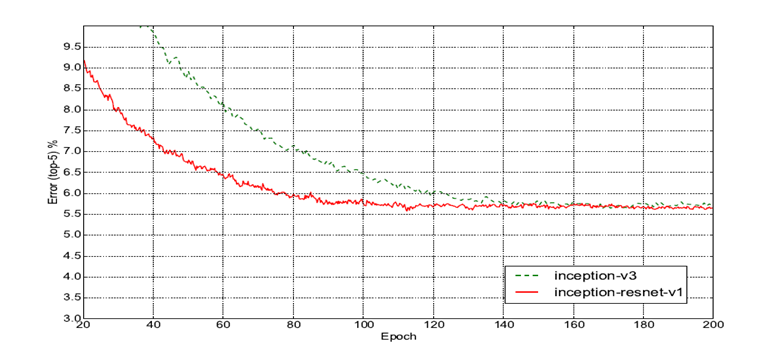
Figure 7. Top-5 error rate comparison between Inception-v3 and Inception-ResNet-V1 based on the ILSVRC-2021 validation set [13].

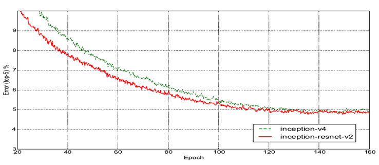
Figure 8. Top-5 error rate comparison between Inception-v4 and Inception-ResNet-V2 based on the ILSVRC-2021 validation set [13].

Table 2. Error rate of each model [13].

From the experiments above, especially in Table 2, the residual inception model merely improves the accuracy rate slightly. Its strongest quality is speeding up the process of training. Both residual inception model v1 and v2 can reach some lower error rate faster than the pure inception models.

3.2.Lightweight Model

Although the large-scale CNN models nominated above are excellent on accuracy rate, they still exist some problem on the device’s memory and processing speed. One large scale model, like ResNet-152, contains plenty of weight parameters through hundreds of layers. It is a heavy burden on memory, whatever it is the time tuning weights or storage the trained weights. What’s more, the processing speed in another challenge for every large-scale models. In realistic, the applications often response to user within milliseconds as a unit. If CNN models require to walk away from the laboratory, the solution is either using better processors or reducing the overall quantity of calculations.

The more advisable solution is to reduce the number of parameters as well as stabilize the accuracy of models. From the publish of MobileNet, it brings a new idea to achieve the above requirement. They name it as ‘Depthwise Convolutional Filters’ [7]. Regular CNN models use the standard filters. The number of channels on filters depends on its input feature map. The number of channels on output feature maps is accordant with the quantity of filters.

Contrast to regular method, depthwise convolutional filters set up the number of filters rely on the number of channels on input feature map. If the input feature map is (5 * 5 * 3), there are 3 separate convolutional filters which have the size (x * x * 1). The number of channels on output feature map depends how many pointwise convolutional filters use after depthwise convolutional filters. For example, the output feature map needs 256 channels, the previous convolutional layer should have 256 pointwise convolutional filters as demonstrated in Table 3.

Table 3. Quantity of calculation steps comparison between regular convolutional filters and depthwise convolutional filters.

3.2.1.ShuffleNet-v2

ShuffleNet-v2 is one of the lightweight models produced in 2018 [14]. It clarifies the relationship between memory access cost and time cost. More specifically, there is a balance point on the number of efficiency (FLOPs and parameters) and accuracy (depth and width). After the experiment on finding this balance point, its researching team offer four guidance as the advice to design a high efficiency model, thereby the production (ShuffleNet-v2) improves compared to the early lightweight model.

The first guidance is equal channel width minimizes memory access cost (MAC) [14]. Most modern models use the architecture of depthwise convolutional filter. Its benefit is to reduce the number of parameters. In this architecture, the pointwise convolutional filter occupies the largest proportion of the calculation steps.

There is an experiment to discuss how the number of channels on input/output feature maps affect the memory access cost. In Table 4, c1 and c2 are the number of channels on input/output feature maps separately. The ratio of c1 and c2 changes on each validation. Finally, the best case is when the numbers of channels are equal. The rest three guidance are ‘Excessive group convolution increases MAC’, ‘Network fragmentation reduces degree of parallelism’, ‘Element-wise operations are non-negligible’ [14]. Followed by these four guidance, ShuffleNet-v2 gathers the operator ‘concat’, ‘channel shuffle’ and ‘channel split’ into a new operator named ‘element-wise operator’.

Table 4. Validation experiment for this guidance [14].

3.2.2.EfficientNet

ShuffleNet tries its best to find the smallest cost on memory access to release the stress on the hardware (such GPU). EfficietnNet focuses on the other point of view to improve the efficiency of the model. Based on the factors of image resolution, depth and width, the establish of EfficientNet wants to find a balance among these three factors [8].

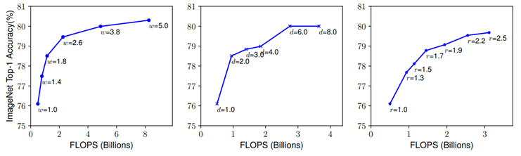
Figure 9. Scaling up the same model with different width (w), depth (d), resolution (r) [8].

In figure 9, it displays the tendency when tuning the width, depth, resolution separately, but the accuracy rate is saturate when it reaches around 80%. As a result, the scaling up on single dimension has a limitation. Thereby, EfficientNet decide to make a method of compound scaling, which could adjust three dimensions in meantime.

In this method, the compound coefficient φ is used to scale the width, depth, resolution: depth: d = α^φ; width: w = β^φ; resolution: r = γ^φ [8].

If the depth doubles in the network, the FLOPs double as well. The width of network and image resolution scaling up one time, the FLOPs cost increases by four times. Therefore, the FLOPs are proportional to (α · β² · γ²).

From B0 to B7, results in Table 5 demonstrate various compound scaling coefficient φ.

Table 5. Result of different EfficientNet model with fixed hyperparameter pair (α-1.2, β-1.1, γ-1.15) based on ImageNet dataset [8].

4.Results

Table 6 shows the result comparison of the aforementioned models. ResNet-RS and EfficientNet-B7 have the highest top-1 accuracy, but the difference of number of parameters is large.

Table 6. Result comparison.

5.Discussion

From the birth of pure ResNet architecture, the idea of scaling up realizes. Then, some other outstanding blocks within the model come out in succession. Many experiments start to hybrid various framework and strategies to continuously improve the model. The model ‘ResNet-RS’ is one of the examples described above which exposes its yielding. The large-scale model traps itself into the laboratory because only the device in the lab with enough budgets can support its work. The invention of lightweight models remedies the weakness of large-scale models. But the accuracy rate does not perform well because the lost of parameters ultimately reduce the ability to capture the feature from inputs. Finally, the upcoming models, such EfficientNet, start to study on the balance of depth, width, and image resolution.

6.Conclusion

In this paper, the comparison among various architectures based on the same dataset (ImageNet). EfficientNet has the highest top-1 accuracy rate and the fewest parameter. It satisfies with the original intention of lightweight models, fewer parameters, and high accuracy rate. The problem that EfficientNet faces is too expensive for most ordinary people to train or expand. Throughout the evolution of CNN models, one reasonable way to set up a better CNN model is to keep the scale of models and make use of every limited parameter by different strategies. With the development of hardware technology in the future, the upgrade on memory and processors will extremely liberate the limitations of CNN models.

References

[1]. Krizhevsky, A., Sutskever, I., & Hinton, G. E. (2012). Imagenet classification with deep convolutional neural networks. Advances in neural information processing systems, 25, 1-9.
[2]. Simonyan, K., & Zisserman, A. (2014). Very deep convolutional networks for large-scale image recognition. arXiv preprint arXiv:1409.1556.
[3]. Szegedy, C., Liu, W., Jia, Y., Sermanet, P., Reed, S., et al. (2015). Going deeper with convolutions. In Proceedings of the IEEE conference on computer vision and pattern recognition, 1-9.
[4]. He, K., Zhang, X., Ren, S., & Sun, J. (2016). Deep residual learning for image recognition. In Proceedings of the IEEE conference on computer vision and pattern recognition, 770-778.
[5]. Szegedy, C., Vanhoucke, V., Ioffe, S., Shlens, J., & Wojna, Z. (2016). Rethinking the inception architecture for computer vision. In Proceedings of the IEEE conference on computer vision and pattern recognition, 2818-2826.
[6]. Iandola, F. N., Han, S., Moskewicz, M. W., Ashraf, K., Dally, W. J., & Keutzer, K. (2016). SqueezeNet: AlexNet-level accuracy with 50x fewer parameters and< 0.5 MB model size. arXiv preprint arXiv:1602.07360.
[7]. Howard, A. G., Zhu, M., Chen, B., Kalenichenko, D., Wang, W., Weyand, T., ... & Adam, H. (2017). Mobilenets: Efficient convolutional neural networks for mobile vision applications. arXiv preprint arXiv:1704.04861.
[8]. Tan, M., & Le, Q. (2019). Efficientnet: Rethinking model scaling for convolutional neural networks. In International conference on machine learning, 6105-6114.
[9]. Deng, J., Dong, W., Socher, R., Li, L. J., Li, K., & Fei-Fei, L. (2009). Imagenet: A large-scale hierarchical image database. In 2009 IEEE conference on computer vision and pattern recognition, 248-255.
[10]. Image Classification on ImageNet. URL: https://paperswithcode.com/sota/image-classification-on-imagenet. Last Accessed: 2023/09/27.
[11]. Bello, I., Fedus, W., Du, X., Cubuk, E. D., Srinivas, A., et al. (2021). Revisiting resnets: Improved training and scaling strategies. Advances in Neural Information Processing Systems, 34, 22614-22627.
[12]. Hu, J., Shen, L., & Sun, G. (2018). Squeeze-and-excitation networks. In Proceedings of the IEEE conference on computer vision and pattern recognition, 7132-7141.
[13]. Szegedy, C., Ioffe, S., Vanhoucke, V., & Alemi, A. (2017). Inception-v4, inception-resnet and the impact of residual connections on learning. In Proceedings of the AAAI conference on artificial intelligence, 31(1), 4278-4284.
[14]. Ma, N., Zhang, X., Zheng, H. T., & Sun, J. (2018). Shufflenet v2: Practical guidelines for efficient cnn architecture design. In Proceedings of the European conference on computer vision, 116-131.
Cite this article
Zhao,Z. (2024). A comparative study of large-scale and lightweight convolutional neural networks for ImageNet classification. Applied and Computational Engineering,47,101-110.
Data availability
The datasets used and/or analyzed during the current study will be available from the authors upon reasonable request.
Disclaimer/Publisher's Note
The statements, opinions and data contained in all publications are solely those of the individual author(s) and contributor(s) and not of EWA Publishing and/or the editor(s). EWA Publishing and/or the editor(s) disclaim responsibility for any injury to people or property resulting from any ideas, methods, instructions or products referred to in the content.
About volume
Volume title: Proceedings of the 4th International Conference on Signal Processing and Machine Learning
© 2024 by the author(s). Licensee EWA Publishing, Oxford, UK. This article is an open access article distributed under the terms and
conditions of the Creative Commons Attribution (CC BY) license. Authors who
publish this series agree to the following terms:
1. Authors retain copyright and grant the series right of first publication with the work simultaneously licensed under a Creative Commons
Attribution License that allows others to share the work with an acknowledgment of the work's authorship and initial publication in this
series.
2. Authors are able to enter into separate, additional contractual arrangements for the non-exclusive distribution of the series's published
version of the work (e.g., post it to an institutional repository or publish it in a book), with an acknowledgment of its initial
publication in this series.
3. Authors are permitted and encouraged to post their work online (e.g., in institutional repositories or on their website) prior to and
during the submission process, as it can lead to productive exchanges, as well as earlier and greater citation of published work (See
Open access policy for details).