1. Introduction

Financial assets, which are essential component of the wealth of individuals, businesses and governments, are also an important support for economic development. Investing in financial assets, especially stocks, bringing high rewards with high risks. Thus, to prevent potential risks and maximize profit acquisition, forecasting the trend of their price fluctuations is particularly important for investors. What’s more, financial institutions can provide better financial services and risk management programs to their clients by predicting financial market movements. Decades ago, analysts judged the return on assets by using logical model. This tactic, however, is less effective because financial markets have unique characteristics like noise, volatility, anomalies, and irregular movements [1]. Then time series analysis models become popular among scholars. These models have limitations in dealing with disruptions and volatility in the stock market system and shows characteristic delay to the origin dataset in some circumstance. To Improve the model, some analysts combined it and neural network. This hybrid model is more efficient and accuracy. Researchers have also experimented with machine learning techniques to predict stock market trends and the result proved that predict movement of stock, this system outperforms some state-of-the-art methods [2].

Here are some introductions of predict models that are popular among the analysts nowadays. When analysing time series data, the statistical method known as autoregressive integrated moving average (ARIMA) is used to represent correlations in the data. When ARIMA is used to build predictive models, it results in better mean error values while maintaining the same mean squared error values as the traditional time series method [3]. Random Forest (RF) are the method based on decision trees in machine learning. Some research indicate that RF typically exhibits higher predictive accuracy compared to individual tree-based classifiers [2]. Artificial neural networks (ANN), often referred to simply as neural networks, are the foundation of deep learning. Recent research on using ANN to forecast the trend of the National 100 Index of the Istanbul Stock Exchange (ISE) reveals extremely high prediction performance with an average correct rate of 75.74% [4]. There is still a drawback of ANN that ANN often exhibits inconsistent and unpredictable performance on noisy data. Support vector machine (SVM), a model used for binary classification, is characterized by a linear classifier with maximal intervals on the feature space as its core structure. But traditional SVM may not as good as ANN [4]. Unlike ordinary feed-forward neural networks, Long Short-Term Memory (LSTM), a unique type of recurrent neural network, may use time series to assess inputs with gating. The results that follow are increasing number of parameters and computational work needed for LSTM due to the introduction of gating and long-term memory mechanisms.

The purpose of this paper is to sort out three different models that categorized as time series analysis models, machine learning models and deep learning models and to analyse the variant model of these three kind of models. The rest of the paper is arranged as follows. Section 2 introduces common inputs for prediction and how to evaluate the prediction. Section 3, 4 and 5 present the principles of ARIMA, Random Forest and Gate Recurrent Unit model, the parameters used and the results obtained separately. Section 6 presents current limitations and future perspectives in this field. Section 7 concludes the paper.

2. Basic description

There are two type of dataset which the researchers always choose as their input set. First is the dataset relating solely and exclusively to the financial asset itself, such as the daily high/low prices, volume records and stock exchange composite index. Analysts more likely to choose those data to analyse short change in market. Unless otherwise specified, this type of dataset is used in all the models in the following sections. Another kind of dataset is the dataset include the business information of both listed company and economic situation of country. To predict long term rewards of equity, the information of what supporting the value of stock are more reliable. Unlike the first type of data which have less pre-processing, because of the second type of data has complex subtype which means there may be interrelationships between them and imbalance in categorization, scholars need to deal with those problem first. Here are some popular parameters to assess the goodness of forecasts. The mean square error (MSE) is a metric that illustrates the degree of discrepancy between the estimated and actual quantities. The formula for the MSE is as follows:

\( MSE=\frac{1}{n} \sum _{i=1}^{n}{({y_{i}}-\hat{{y_{i}}})^{2}} \) (1)

where n denotes the sample size, \( {y_{i}} \) denotes the actual observations, and \( \hat{{y_{i}}} \) denotes the predicted values. MSE squares the error, which makes it particularly susceptible to outliers because its value rises with increasing error. It is able to give appropriate penalty weights to gradients rather than treating them equally. The square root of the mean square error is the root mean square error (RMSE). The formula for RMSE is as follows:

\( RMSE=\sqrt[]{\frac{1}{n} \sum _{i=1}^{n}{({y_{i}}-\hat{{y_{i}}})^{2}}} \) (2)

RMSE has similar characteristics to the MSE, while its calculated result is more intuitive with the same units as the actual value. The mean absolute error (MAE) denotes the mean of absolute errors between predicted and observed values. Due to MAE's ability to eliminate offsetting mistakes, the size of the real prediction error is accurately reflected. MAE's formula is as follows:

\( MAE= \frac{1}{n} \sum _{i=1}^{n}|{y_{i}}-\hat{{y_{i}}}| \) (3)

The MAE calculates the absolute value of the error and is less sensitive to outliers compared to other loss functions such as MSE. The gradient of the MAE is the same for large or small errors, which may lead to slower convergence of the model during training. The related metric known as mean absolute percentage error (MAPE) actually refers to the MAE scale as a percentage unit rather than a unit of the variable. Following is the MPAE formula:

\( MAPE= \frac{1}{n} \sum _{i=1}^{n}|\frac{{y_{i}}-\hat{{y_{i}}}}{{y_{i}}}| \) (4)

MAPE has similar properties to MAE and MAPE is more sensitive to outliers.

3. ARIMA

The shape of the ARIMA model is denoted by the general notation of ARIMA (p, d, q). ARIMA treats the forecast object's data series as a stochastic sequence, and this stochastic sequence can be approximately characterized by a specific mathematical framework. The future values of the past and present values of the time series can be predicted once this model has been comprehended. In recent research about comparing ARIMA and LSTM on forecasting NASDAQ stock exchange [5], the researchers attempted to use Nasdaq stock price movement trend data from different industries as an input dataset. The input data is finally organized into a table with two columns for timestamps and stock prices. Scholars build the ARIMA model according to the Box-Jenkins method which can totally divided into 3 stages. In the first stage, the identification stage, the characteristics of the time series being analysed are examined to check their relationship. In the second stage, the estimation and testing stage, the parameters of the selected model are estimated. There also need a diagnostic check and analyse model residuals. In the third stage, the model is used for prediction where the dataset will be divided into in-sample and out-of-sample and the input data also need to be logarithm zed in order to obtain the desired series smoothness.

The result show that compared to the LSTM method, ARIMA performs well (lower MAPE) for training data time ranges of one month, three months, and nine months. Because the ARIMA model is one of the fundamental models in time series analysis, it is also employed in a variety of mixed applications, including the forecasting of carbon futures prices using the ARIMA-CNN(Convolutional Neural Networks)-LSTM model [6] and the ARIMA-SLFNs(Single Layer Feedforward Neural Network) model [7]. The hybrid ARIMA-CNN-LSTM model captures data with the type of both linear and nonlinear features by combining CNN and LSTM layers with the ARIMA model [6]. In the construction of the this model, ARIMA is used to get linear attributes. CNN captures hierarchical data structure, whereas LSTM captures long-term dependencies in the data. Figure 1 depicts the CNN-LSTM model's structure.

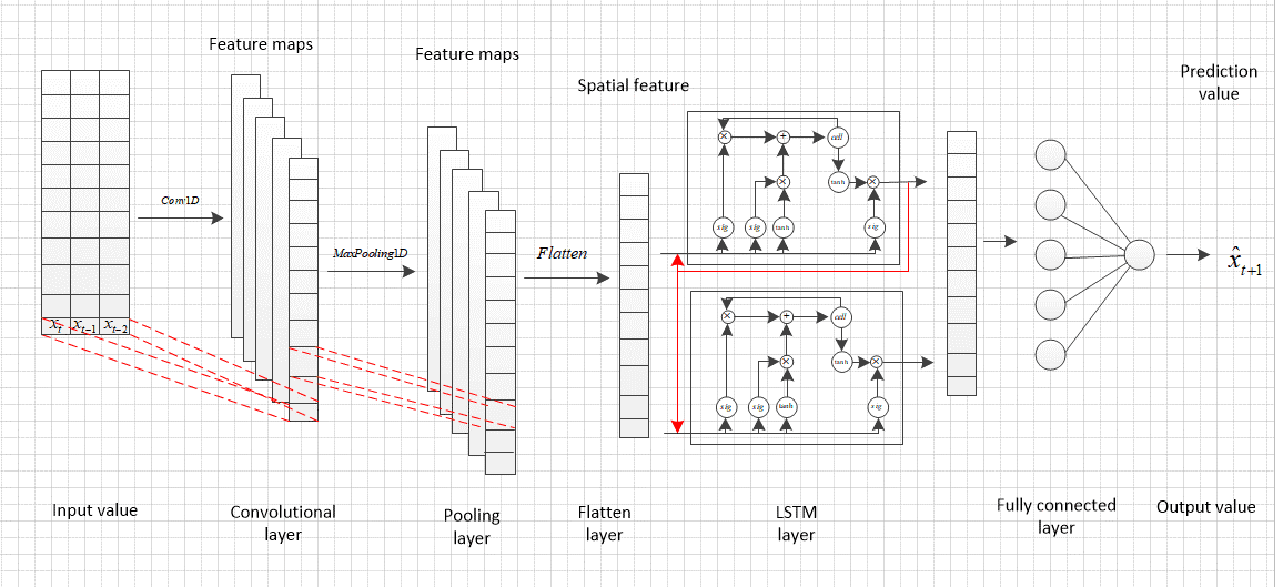
Figure 1. The CNN-LSTM model's construction [7].

The outcomes demonstrate that the ARIMA-CNN-LSTM model can predict outcomes more precisely than the basic model in terms of RMSE and MAPE performance indicators. The ARIMA-SLFNs model is made up of the filter, ARIMA model, decomposition pools, and different SLFN models [7]. The raw carbon price is first separated into linear component and nonlinear residue before further decomposing into IMFs. Then, using the BOA-based SLFNs model based on the actual data of the residual IMFs and a single-period lag, the ARIMA forecasts are nonlinearly adjusted. Figure 2 shows the general construct in detail. Researchers investigated filter mixing models for several SLFNs and discovered that HP(Hodrick Prescott)-ARIMA-KELM(Kernel Extreme Learning Machine) outperformed the other models in terms of predictive accuracy, generalization, and forecasting power across two distinct datasets.

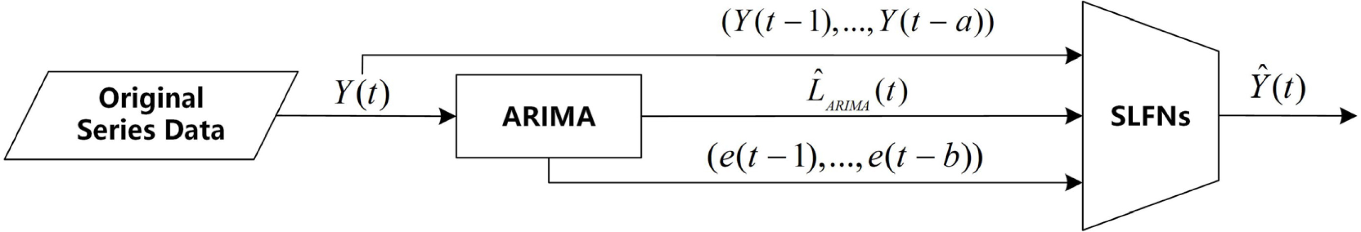
Figure 2. The parallel–series hybrid structure [7].

4. Random forest

The Random Forest (RF) algorithm uses the Bagging concept of integrated learning to integrate numerous trees. Its fundamental building block is the decision tree, and it makes extensive use of "trees" to create "forests." The word “Random” has two means, one is random choosing sample in training set to each tree, another is random choosing feature dimension to segment the nodes with the best features from these feature dimensions. Those features of RF make sure this model less prone to overfitting and have good noise immunity. In recent research of using mixture RF model to forecast stock price trend [8], researchers try to compare RF method and support vector machine (SVM). These programs are used to determine if the cost of a stock is higher than the cost on a given date in order to develop a profitable trading strategy. In this paper, scholars use Profit unity method to frame the example elements to the acknowledgment framework. The result shows that when using the provided dataset, the RF Model outperforms the SVM. Nonetheless, support vector machines are an excellent substitute for financial estimation when the information is in a time schedule design. There may be a variety of components that can affect the forecast execution of a model used for stock market forecasting.

Researchers projecting cryptocurrency assets in futures markets in another paper [9]. Here, RF is used to analyse three scenarios in relation to input variables, including candlestick patterns, technical indicators, and both at once. Candlesticks show price changes over time, which can last anything from a few seconds to a month. For each range, volume and Open, High, Low and Close (OHLC) data are supplied. The findings show that test phase data and out-of-sample predictions were highly variable, but that the greatest outcomes were finally obtained when 1-day intervals were combined with candlestick morphology as a feature, rather than producing the required horizontal line. Here is also a hybrid LSTM-RF model [10]. LSTM-RF, which is consist of plural components LSTMs, used the average values of those components as the outputs. The set of training data and input variables for each LSTM are chosen at random for the duration of the training cycle from the entire dataset. By employing LSTM to create classifiers or regressors rather than decision trees in RF, it blends LSTM with RF. Numerous input variables can be handled by RF without overfitting. LSTM, however, performs better than temporal pattern decision trees. Given the benefits of both approaches, the overfitting issue can be minimized in the proposed model because each LSTM makes use of a significantly smaller number of variables than the total. Finally, the researchers contrasted the LSTM-RF model with the fundamental RF and LSTM models. and the LSTM-RF model outperforms RF in terms of temporal pattern learning, and the proposed model prevents overfitting while learning efficiency is better than LSTM. Additionally, though the deep learning model is normally a black-box model, the LSTM-RF model is interpretable due to its use of variable significance analysis of RFs.

5. GRU

A subtype of recurrent neural networks (RNNs) is the gate recurrent unit (GRU). Similar to LSTM, it is also meant to overcome problems with long-term memory and gradient in backpropagation. The use of GRU can result in results that are comparable to LSTM and is easier to train. This has the potential to greatly improve training effectiveness.

In a recent paper about forecasting oil price with hybrid GRU model [11], scholars combine GRU with a decomposition-reconstruction method, variational modal decomposition (VMD) method. Using decomposition-reconstruction techniques, the original time series is divided into multiple independent components, each of which is predicted independently, and the outcomes are then integrated. VMD is utilized in the hybrid VMD-GRU model to eliminate redundant information from the signal and lower the error level. The general constructure of VMD-GRU is illustrated in figure 5. Moreover, the sample entropy (SE) approach is also used to guarantee adequate signal decomposition-reconstruction, and researchers ultimately design a hybrid VMD-SE-GRU model. Figure 6 shows the hybrid model’s overall construction. When those two hybrid model are compared, the multivariate model which combined with SE has the lowest run time but was the least effective—it could only provide a general trend and was unable to adequately match high volatility parts. Although the univariate hybrid model combined with SE has half the run time of the hybrid model without SE, it is marginally less efficient than the hybrid model without SE in terms of capturing the troughs in the data.

In addition, hybrid GRU models have better accuracy and shorter runtime compared to hybrid LSTM and DNN models. In the meantime, this hybrid GRU framework is a powerful oil prediction framework with good prediction performance, fast computation times, and resilience to various oil indices when the trade price curve is smoother. Another paper mentions a new hybrid model based on GRU [12]. Scholars have proposed a StockNet network to overcome the overfitting problem in the machine learning process. The injection block injects unique features one by one, and the survey block utilizes the index features as input for equity index forecasting. The general constructure of StockNet is illustrated in Figure 3. In the StockNet system, a fully connected layer called FC is added after the GRU layer has processed the input features. The data is transferred via several fully connected layers in the studied and injected sub-models before the outputs of the two sub-models are integrated utilizing the fully connected layers. For target prediction, the value of the final completely connected layer is determined. The results show a significant decrease in MSE, MAE and MAPE compared to the ModAugNet method (an LSTM model with overfitting prevention) without overfitting. Here is another hybrid model based on GRU [13]. The VIX-Lasso-GRU model builds on GRUs by incorporating VIX(volatility index) data and the least absolute contraction and selection operator (Lasso) technique. In this model, the VIX information is a proxy for implied volatility which is used as a predictor. Lasso's algorithm can enhance the model's forecasting performance by reducing the noise from datasets and can also lower dimensionality of data. The general constructure is illustrated in Figure 4. The outcomes demonstrate that the addition of VIX greatly increases prediction accuracy and that by choosing useful features, the Lasso technique can reduce training time.

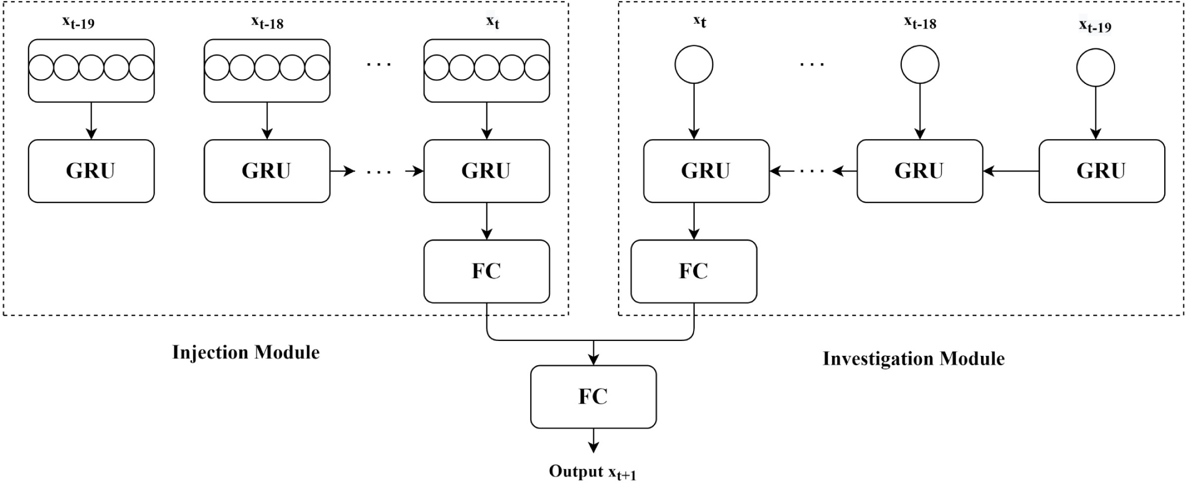
Figure 3. StockNet proposed architecture [12].

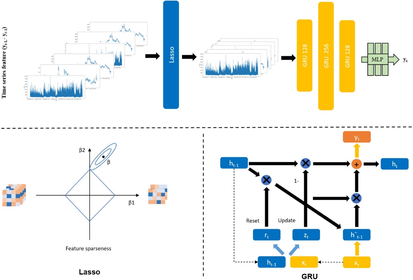
Figure 4. The frame for the VIX-Lasso-GRU model [13].

6. Limitations and prospects

Although machine learning has made significant improvements in financial asset forecasting accuracy and efficiency, all current forecasting methodology still have their limitations. First, the noise interference, the data quality and the overfitting are three major factors which influence the accuracy of forecasting and none of these can be completely avoided when using machine learning algorithms. Second, some predictions made by models that only use machine learning are incomprehensible. The collection of operations the model does when making a forecast is unknown, or even if a person is aware of every action the model takes during the decision-making process, the operations cannot be explained in terms of semantics that a human can comprehend. Third, those models built by academics can only forecast for a particular type of financial asset in a particular market. The model is no longer valid when it is applied to other markets or to another financial asset. Thus, the effects of those models sometimes are not comparable because they work better in their own specific contexts.

For a given model, they all have their own limitations. For the time series model ARIMA, it requires the time series data to exhibit high smoothness and homoskedasticity. If these requirements are not met, the model's predicting ability will be adversely affected. Therefore, ARIMA may not be the most reliable option for predicting volatile equities due to its sensitivity to non-smooth and heteroskedastic data patterns. For the Random Forest algorithm, it should be noted that regression analysis is constrained within the range of the training set data. This limitation can lead to overfitting issues when dealing with data that contains specific types of noise. In other words, if the training data is not representative of the true population, the model may fit too closely to the noise in the training set and fail to generalize well to new observations. For the GRU model, though it is an efficient model for processing lengthy sequences, it may encounter similar challenges as other recurrent neural network types, such as the problem of gradient vanishing. This means that when backpropagating errors through the network, the gradients may exponentially diminish, making it difficult for the GRU model to capture long-range dependencies accurately. Therefore, while GRU is suitable for processing long sequences, it is important to monitor and mitigate the potential issue of gradient vanishing. Organizing of those researches suggests that future financial asset analysis should incorporate machine learning algorithms to further enhance interpretability. Meanwhile the combination of time series analysis algorithms and deep learning algorithms proves the significant role of this hybrid model in financial asset analysis.

7. Conclusion

To sum up, the combination of financial asset forecasting and machine learning has proven to be a proven approach. Some of the more popular methods applied to financial asset forecasting in recent years are methods such as ARIMA, RF, GRU and their respective hybrid models. Models that use the ARIMA algorithm to capture linear elements and use deep learning methods to predict trends have shown good results, RF algorithms have shown good results in dealing with data noise and in terms of interpretability, and GRU has achieved good results in terms of forecasting efficiency. However, deep learning methods currently still have the limitation of being non-interpretable. At the same time, the models that scholars are currently working on can only be effective in predicting specific types of assets in specific market environments, and it is still difficult to generalize these models to a wider range of predictions. This study illustrates future research directions in the field of financial asset forecasting by analysing and organizing the characteristics of three different mainstream models.

References

[1]. Kehinde T O, Chan F T S and Chung S H 2023 Expert Systems with Application vol 213 p 119299.
[2]. Toochaei M R and Moeini F 2023 Expert Systems with Applications vol 213 p 119186.
[3]. Tao L Z 2022 Business Economy Research vol 5(5) pp 38-45.
[4]. Kara Y, Boyacioglu M A and Ömer K B 2011 Expert Systems with Applications vol 38(5) pp 5311-5319.
[5]. Kobiela D, Krefta D, Kr ́ol W and Weichbroth P 2022 Proce-dia Computer Science vol 207 pp 3836-3845.
[6]. Ji L, Zou Y, He K and Zhu B 2019 Procedia Computer Science vol 162 pp 33-38.
[7]. Qin Q, Huang Z, Zhou Z, Chen Y and Zhao W 2022 Applied Soft Computing vol 119 p 108560.
[8]. Illa P Km, Parvathala B and Sharma A K 2021 Materials Today: Proceedings vol 56 pp 1776-1782.
[9]. Orte F, Mira J, S ́anchez M J and Solana P 2023 Research in International Business and Finance vol 64 p 101829.
[10]. Park H J, Kim Y and Kim H Y 2022 Applied Soft Computing vol 114 p 108106.
[11]. Zhang S, Luo J, Wang S and Liu F 2023 Expert Systems with Applications vol 218 p 119617.
[12]. Gupta U, Bhattacharjee V and Bishnu P S 2022 Expert Systems with Applications vol 207 p 117986.
[13]. Fang W, Zhang S and Xu C 2023 Expert Systems with Applications vol 219 p 121968.
Cite this article
Li,Y. (2024). Financial assets prediction based on ARIMA, Random Forest and GRU. Applied and Computational Engineering,50,149-156.
Data availability
The datasets used and/or analyzed during the current study will be available from the authors upon reasonable request.
Disclaimer/Publisher's Note
The statements, opinions and data contained in all publications are solely those of the individual author(s) and contributor(s) and not of EWA Publishing and/or the editor(s). EWA Publishing and/or the editor(s) disclaim responsibility for any injury to people or property resulting from any ideas, methods, instructions or products referred to in the content.
About volume
Volume title: Proceedings of the 4th International Conference on Signal Processing and Machine Learning
© 2024 by the author(s). Licensee EWA Publishing, Oxford, UK. This article is an open access article distributed under the terms and
conditions of the Creative Commons Attribution (CC BY) license. Authors who
publish this series agree to the following terms:
1. Authors retain copyright and grant the series right of first publication with the work simultaneously licensed under a Creative Commons
Attribution License that allows others to share the work with an acknowledgment of the work's authorship and initial publication in this
series.
2. Authors are able to enter into separate, additional contractual arrangements for the non-exclusive distribution of the series's published
version of the work (e.g., post it to an institutional repository or publish it in a book), with an acknowledgment of its initial
publication in this series.
3. Authors are permitted and encouraged to post their work online (e.g., in institutional repositories or on their website) prior to and
during the submission process, as it can lead to productive exchanges, as well as earlier and greater citation of published work (See
Open access policy for details).