1. Introduction

The real estate industry is crucial for economic development and societal progress, reflecting the aspirations of individuals and families and the overall economic health of a region. A. H. Maslow states in A Theory of Human Motivation: “Undoubtedly these physiological needs are the most pre-potent of all needs” (1943, p.374) [1]. Among physiological needs, shelter (house), as a necessity, is essential for people. Hence, it is essential for people like policymakers, real estate professionals, and homeowners to comprehend the factors that influence housing prices. In this context, the study of house price prediction has gained significant attention, given its potential to offer insights into the factors that drive housing market fluctuations and their importance for various stakeholders.

This paper focuses on the task of house price prediction in King County, Washington. King County, situated in the heart of the Pacific Northwest, represents a diverse and dynamic real estate market, characterized by a mix of urban, suburban, and rural areas. With its vibrant economy, cultural attractions, and natural beauty, King County has drawn a diverse population, contributing to the complexity of its housing market. It is the most populated county in Washington and the 13th largest populated county in the US [2]. According to Maslow’s hierarchy of needs, the base level of the pyramid is physiological needs, which include shelter. Thus, there is currently a significant need for residential properties in King County.

The importance of precise price predictions in the real estate market is profound, as these forecasts have the potential to significantly influence the decisions of a multitude of stakeholders, including prospective homebuyers, sellers, real estate agents, investors, and policymakers. An accurate and reliable predictive model is, therefore, a cornerstone of informed decision-making in the housing industry.

This research goes beyond previous economic analysis and uses well-founded models in machine learning to explore this problem. Four supervised learning models, linear regression, RF, ANN and XGBoost will be used to predict the relationship between different features of the house and the price of the house. The result will conclude the important features that influence the house price. This will provide a guide for future house purchases or investments.

The following is how the paper is organized: The section 2 will go over our data processing, including data selection and pre-processing. Section 3 is about the methodology of our research. It will include the four models we used to process our data. Section 4 will illustrate further experiments based on the results produced by our models. Finally, the conclusions are in section 5.

2. Data Processing

2.1. Data Preprocessing

The "House Sales in King County, USA" [3] dataset contains 21,611 pieces of data and 21 features representing house prices from May 2014 to May 2015. These features (except the price itself), were used to predict the house price.

The next step is to investigate and clean the dataset. Features with missing data will be removed (we are unable to interpolate the method to insert values because of its randomness). Also features such as id and date will be dropped, because they are apparently subjective factors that will not fit the objective prediction of house price.

Since there are unit differences in feature data, failure to standardize it will lead to a decrease in accuracy and speed of model training. So the standardization of the data is to make sure that the data is on a relatively similar scale. Its goal is to transform the data into a normal distribution with a mean and standard deviation of 0 and 1, respectively. The formula that follows can be used to express standardization:

\( Z=\frac{Xi-μ}{σ} \) (1)

After the process with the dataset and features, the final dataset contains 21,611 data with 19 features (including price), 6 of which are categorical values and 12 of which are numerical values. Remove examples 12 and 19 due to the absence of sqft_above feature. Additionally, exclude the features id and date on account of subjectivity. Each property is described in depth in Table 1.

Table 1. List of Attributes (list few important attributes)

2.2. Data Analysis

Data exploration is a crucial phase in the prediction model that may assist choose the best model more precisely. Also, the exploration will help the researchers to easily find the inherent link among data.

Figure 1 shows the distribution of different grades in the King County region. Also with the Lat, Long, Price, and Year information. (We just show the Grade 8-12 distribution here). From Figure 1, the map shows the houses distributed in the coastal areas are generally of higher grade and density. Besides, Figure 2 (Blue being cheap and red being expensive) shows the price distribution in the King County region. It becomes clear from this map that house prices are higher in the downtown area (near Elliott Bay in the top left of the map) and in Redmond (east of Lake Washington). House prices are intermediate north and south of downtown. In addition, we can see that waterfront property is more expensive [4].

In addition, Figure 3 gives the correlation between different features, which clearly shows the degree of the correlation by judging the color. More specifically, Figure 4 shows the features whose correlation is all greater than 0.5 which has a big positive influence on the house price.

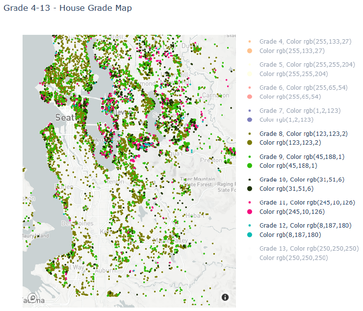
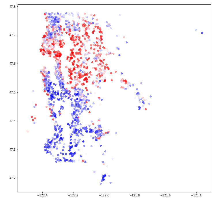
Figure 1. Grade Distribution (Original) Figure 2. Price Distribution (Original)

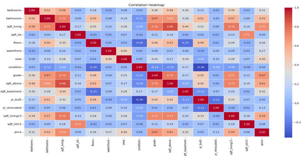
Figure 3. Features correlation heatmap (Original)

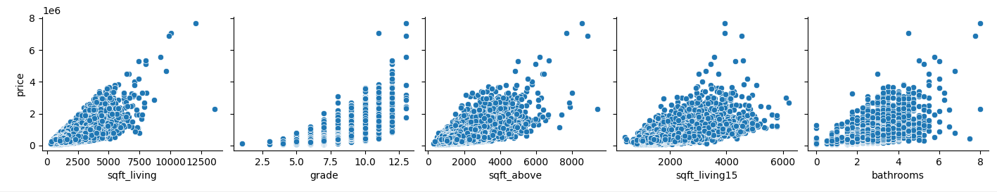
Figure 4. Features correlation > 0.5 (Original)

3. Methodology

3.1. Linear regression (LR)

Linear regression is a method employed to establish relationships between a dependent variable and one or more independent variables. The linear regression model's connection may be used to predict the dependent variable by varying the independent variables. It is a very efficient and effective model to help predict the relationships in machine learning.

Linear regression encompasses two principal forms: simple linear regression, applicable when there is only one independent variable, and multiple linear regression, employed when there are multiple independent variables. In the situation of house price prediction, because there are multiple features that may influence the house price, a multiple linear regression model will be deployed.

The hypothesis of the linear regression model is as follows:

\( {h_{θ}}(x) = {θ_{0}} + {θ_{1}}{x_{1}} + {θ_{2}}{x_{2}}+...+ {θ_{n}}{x_{n}} \) (1)

where h is the target, which is the price of the house. \( {x_{1}} \) , \( {x_{2}} \) , …, \( {x_{n}} \) are the independent variables or features, and \( {θ_{0}} \) , \( {θ_{1}} \) , \( {θ_{2}} \) , …, \( {θ_{n}} \) are the coefficients of the independent variables \( {x_{1}} \) , \( {x_{2}} \) , …, \( {x_{n}} \) .

The target of this analysis will be the price of the house, which will be presented in the training dataset. The whole linear regression model aims to fit a curve to the provided dataset while minimizing errors [5].

3.2. Random forest (RF)

RF is a type of ensemble model that aggregates numerous decision trees' predictions to produce a more precise ultimate forecast. Based on prior research, RF algorithm is a proven strong technique [6]. S. Raschka and V. Mirjalili summarised the RF method in the following procedures [7]:

1. Create a random bootstrap sample of size n (choose n house price samples at random from the training set with replacement).

2. 2. Create a decision tree from the bootstrap sample, using the following nodes:

(a) Select d house features at random (from a total of 18 house features in our research) without substitution.

(b) Divide the node using the feature that offers the optimal split based on the objective function, such as maximizing information gain.

3. Repeat the procedure 1–2 k times more.

4. Use the majority vote to give the class label based on the predictions of each tree.

To train the model in this study, we followed the methods outlined below:

Creating a Random Forest Regression Model: We utilize the RandomForestRegressor class from the sklearn library to create a random forest regression model.

Using RandomForestRegressor method from the sklearn library to choose the best combination of parameters:

'n_estimators': 200, 'min_samples_split': 5, 'min_samples_leaf': 1

Model Training: We train the random forest regression model using the training dataset.

Model Prediction: We use the test dataset to make predictions with the trained model, obtaining predicted house prices.

3.3. Artificial Neural network (ANN)

The artificial neural network (ANN) is a supervised learning approach that is based on the operation of neural networks that are biological [8]. It is made up of synthetic neurons, each of which can receive input and output signals from several other neurons.

Neurons are usually divided into several layers. The input is transferred from the input layer to the output layer through several layers. Neural networks are frequently utilized to tackle a wide range of issues that traditional rule-based programming cannot. Therefore, it is a good comparison object for other methods. In this research, the ANN method is used to compare other methods to show the performance of other methods.

The neural network model used for training has a total of three hidden layers. We performed a total of 500 iterations during training [8]. A multi-layer feedforward neural network with an input layer, three hidden layers, a dropout layer, and an output layer is the structure of the neural network model. The specific parameter in each layer and structure Figure 5 will show below:

• Input Layer:

The input layer's number of neurons equals the number of features. We use our 18 house features here.

• Hidden Layers:

There are three hidden layers with 32, 64, and 128 neurons respectively.

To introduce non-linearity, each hidden layer employs the Rectified Linear Activation (ReLU) function.

• Dropout Layer:

To reduce overfitting, a Dropout layer is inserted after the third hidden layer.

The dropout probability is set to 0.2, which means that during training, each neuron has a 20% probability of being randomly turned off, helping to improve the model's generalization.

• Output Layer:

For regression tasks (predicting housing prices), the output layer is made out of a single neuron.

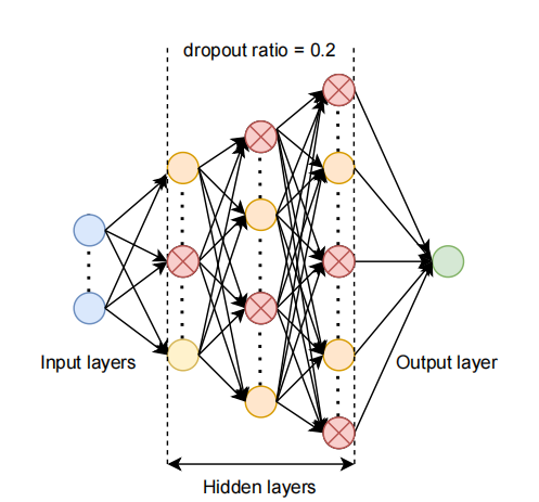
Figure 5. Structure of ANN [8]

3.4. XGBoost

XGBoost is one of the applications in gradient boosting machines (gbm), which is known as one of the top performing supervised learning algorithms. It is applicable to both regression and classification issues [9]. The structure of XGBoost is showed in Figure 6 [10]. The way XGBoost works is as follow as well:

• Initializing the Model:

Initialize a model, typically a decision tree with only one leaf node. The initial leaf node's prediction is set to the average of all target values in the training data:

\( {F_{0}}(x)=\sum {y_{i}}/m \) , where i ranges from 1 to m ( m is the number of training samples, Seven tenths of 21,611 in our research)

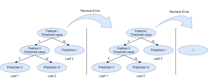
Figure 6. Schematic of Xgboost trees [10]

• Calculating Initial Predictions:

Use the initialized model to calculate initial predictions:

\( {F_{0}}(x)=\sum {y_{i}}/m \) , where i ranges from 1 to m.

• Computing Negative Gradients of the Loss Function:

Calculate the loss function's negative gradients with regard to the present model.

The loss function for regression issues is often mean squared error (MSE):

Negative Gradient \( ({g_{i}})=-∂L({y_{i}},F({x_{i}}))/∂F({x_{i}})={y_{i}}-{F_{0}}({x_{i}}) \) , where i ranges from 1 to m.

• Fitting a New Tree Model:

Fit a new decision tree model to approximate the negative gradients of the loss function. This new tree model is referred to as a "weak learner."

When fitting the new tree model, XGBoost uses first-order and second-order gradient information to select the best splitting points that minimize the loss function.

• Updating the Model:

Update the model by adding the predictions of the new tree model to the previous model:

\( {F_{1}}(x) = {F_{0}}(x) + {η_{1}} * {h_{1}}(x) \) , where \( {h_{1}} \) (x) is the prediction of the new tree model, and η is the learning ratio.

The learning ratio (η) controls the impact of each new model, and it's typically set to a small value. (After using GridSearchCV method from the sklearn library we set the η as 0.1).

• Repeat Steps 3-5:

Repeat the process of calculating negative gradients, fitting a new tree model, and updating the model iteratively until a preset number of repetitions is reached or other stopping requirements are met.

• Introducing Regularization Terms:

Introduce regularization terms, such as L1 and L2 regularization, to control the complexity of the model and prevent overfitting.

Regularization Term \( (Ω(F(x))) = γ * Φ(T) + ½ * λ * Σ({w_{i}}²) \)

Where \( Φ(T) \) represents the number of leaf nodes in the tree (we used get_booster().get_dump() to get the tree structure of the model and len(tree.split('\n')) to count the number of leaf nodes per tree in the research), wᵢ represents the score of each leaf node, and \( γ \) and λ are regularization hyperparameters.

• Model Output:

The final model output is the sum of predictions from all weak learners, each scaled by the learning rate:

\( F(x) = {F_{0}}(x) + {η_{1}} * {h_{1}}(x) + {η_{2}} * {h_{2}}(x) + ... + {η_{t}} * {h_{t}}(x) \) (2)

The final model output is used for making predictions in regression problems.

1. Minimizing the Loss Function:

XGBoost's objective is to minimize the loss function, which includes the loss value and regularization terms.

Objective Function \( (Obj(θ)) = L(y, F(x)) + Ω(F(x)) \) (3)

In our research, we build our model as follow:

2. Build the initial tree model:

When creating an XGBoost regression model, we initializes a model with a simple tree as the baseline model.

3. Iterative training:

GridSearchCV is used to search for the best hyper parameter configuration as part of XGBoost's training process. During the search process, multiple tree models are built and iteratively trained according to the given parameter grid.

The GridSearchCV in the code fits the model for each parameter configuration and calculates the corresponding mean square error (gradient of the loss function). The model building and updating process in these iterations is similar to the training process of XGBoost.

4. Combination of final models:

In the code, grid_search.best_estimator_ is used to get the best model in the search process (combining multiple tree models). The best parameters of the model are obtained: learning_rate: 0.1, max_depth: 4, mid_child_weight:3, n_estimators: 300. This optimal model will be used in the final forecast.

5. Final prediction:

best_xgb_model.predict(X_test) uses the best model to make the ultimate prediction, which involves adding the predictions of multiple tree models and weighting them by the learning rate.

4. Experiment and Analysis

This paper uses kaggle.com to obtain the housing price data of King County in one year and the property characteristics of houses as the experimental objects. Besides, this paper predicts the housing price through the different degree of influence of different property characteristics on the housing price. In the end, after the horizontal comparison of different prediction algorithms, an overall ranking of the influence of house characteristics on house prices is obtained.

4.1. Experiment Details

The dataset will be divided into two parts for the experiment: 70% of the data will be used to train the model, and 30% will be used to test the model.

4.1.1. The Result Of Linear regression. Before running the linear regression model, the relationship between different factors has been analyzed (Figure 7). Most of the relationships between price and the area of different parts of the house are linear, which satisfied the prerequisite for running a linear regression model.

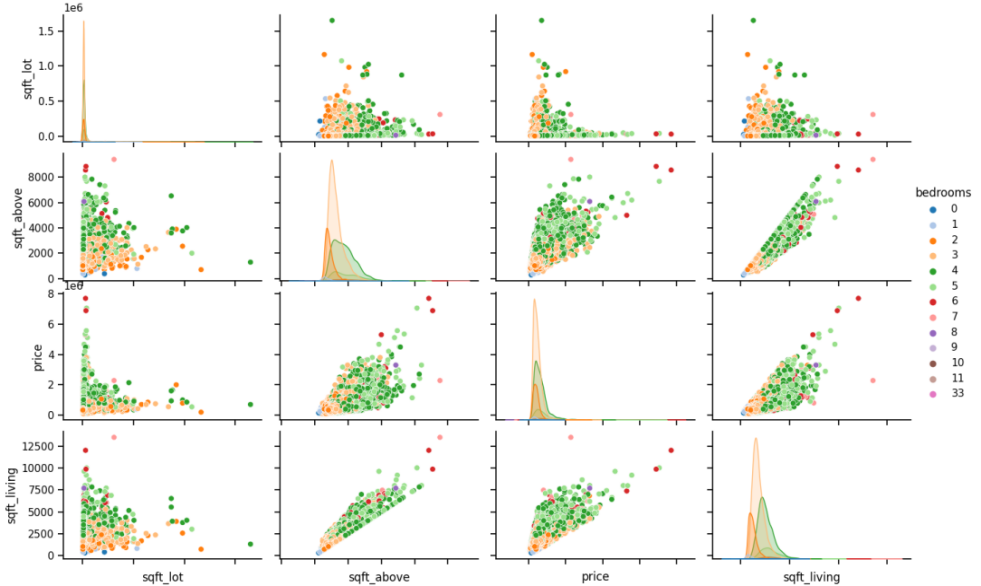
Figure 7. Correlation between price and area (Original)

Following the analysis of the relationship between price and area, a simple LR model for the price and living area of the house was built by using gradient descent to find the minimum cost function (Figure 8).

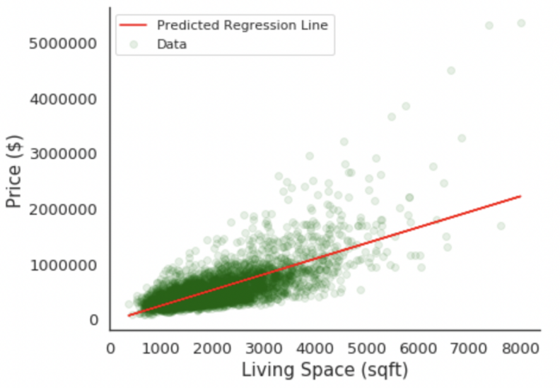
Figure 8. Linear regression model for price and living area (Original)

Subsequently, after evaluating the performance of the simple linear regression model, we proceeded to develop a multiple linear regression model based on our hypothesis using the Ordinary Least Squares (OLS) regression test. The resulting model demonstrated a commendable R-squared value of 0.706, affirming the appropriateness of the linear regression model for this research.

4.1.2. The Result Of Random forest and XGBoost. In the process of hyperparameter optimization of Random Forest and XGBoost models, we use the RandomizedSearchCV function from python's scikit-learn library to achieve better performance of our model. The following two graphs (Figure 9 and Figure 10) show the performance improvement of the two algorithms after 100 iterations. It can be seen that their RMSLE starts to decline significantly and becomes stable at about 80 iterations, and the hyperparameters reach the optimal level.

The result of our research gives an exceptional R-squared value of 0.878 in random forest algorithm and 0.888 in XGBoost algorithm.

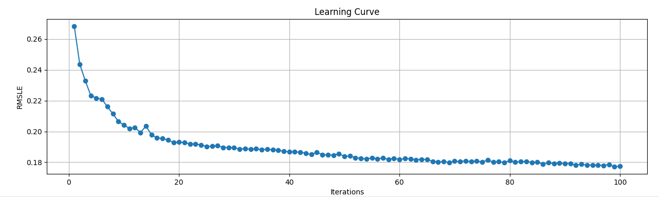
Figure 9. Random Forest Learning Curve (Original)

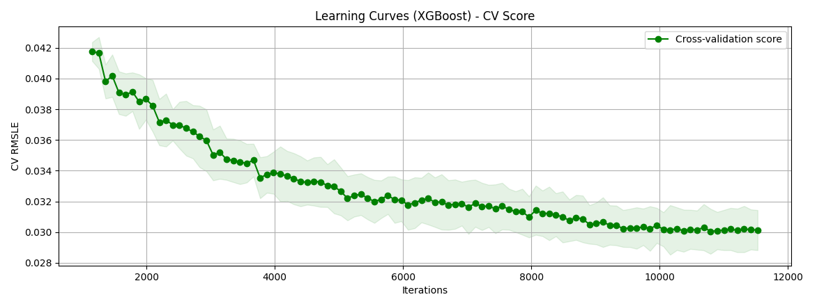
Figure 10. XGBoost Learning Curve (Original)

4.1.3. The Result of Artificial Neural network. In ANN, we use ReLU function as activation function, because its characteristics are helpful to train deep neural networks, and the calculation of ReLU is simpler and more efficient than other activation functions. Because it does not cause gradient disappearance problems, neural networks can be trained more easily. The TensorFlow library is used for hyperparameter optimization.

The Figure 11 below is our training of ANN learning rate to find the best learning rate. It can be seen that when the learning rate is 0.1, the MSE quickly reaches a relatively stable value, but it is easy to miss the local minimum and the best parameter combination. When the learning rate is 0.0001, it takes a long time to reach the relatively stable value of MSE, and the time cost is relatively high. Therefore, we choose 0.001 with moderate decline speed as the learning rate for the configuration of hyperparameters.

The result of the ANN with 0.001 learning ratio gives 0.846 in R-squared value.

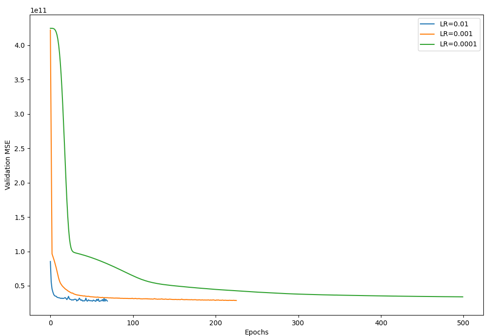
Figure 11. Different learning rates curve (Original)

4.2. Overall comparison

Table 2. Comparison of Accuracy

The above Table 2 shows the comparison between the algorithms that are used in this research, where it is found that XGBoost gives the highest accuracy, 88.8 percent. While the Linear regression is the lowest at 70.6 percent with the Neural network in 84.6 percent and Random forest in 87.8 percent. The degree of fit of the four algorithms is also shown below in Figure 12.

Overall, XGBoost and RF are generally more complex nonlinear models in terms of complexity, and they can better capture complex relationships and nonlinear patterns in the data (because the relationship between house prices and features is generally complex and non-linear). In contrast, linear regression, which performs poorly when dealing with non-linear relationships. ANN is somewhere in between, it can learn nonlinear relationships, but its performance is highly dependent on the choice of network structure and parameter adjustment (given that the neural network in our study only uses a relatively simple three-layer feedforward neural network, the parameters are default, and the amount of data is limited).

High adaptive advantage over integrated methods: XGBoost and RF are both integrated learning methods that improve performance by combining multiple weak learners. This makes them more robust and predictive in modeling, able to deal effectively with noise and outliers.

Properties of the data set itself: Given the complex non-linear relationships, interactions, and importance of features in house price data, XGBoost and RF are often better able to fit these properties. ANN can also learn nonlinear relationships, but requires more data and tuning to maximize its performance, and the number of data sets here may not be enough for ANN to further learn to improve model performance.

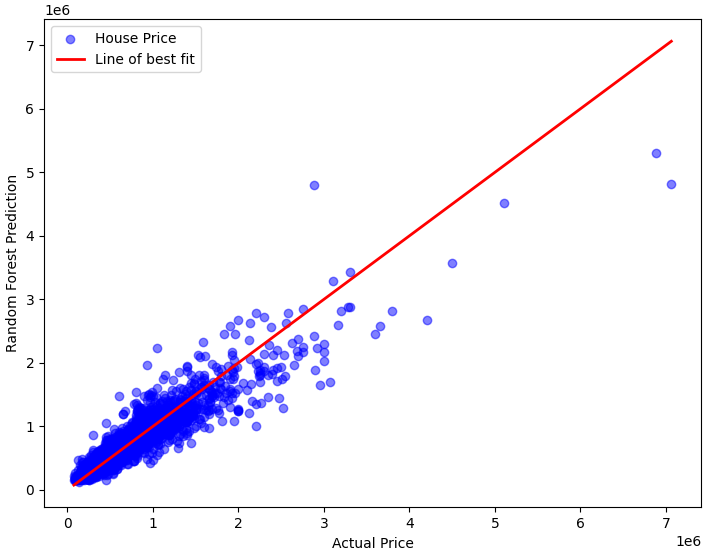
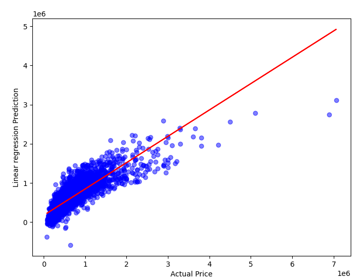
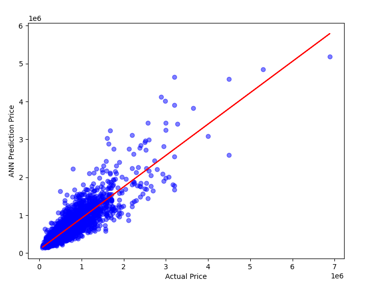
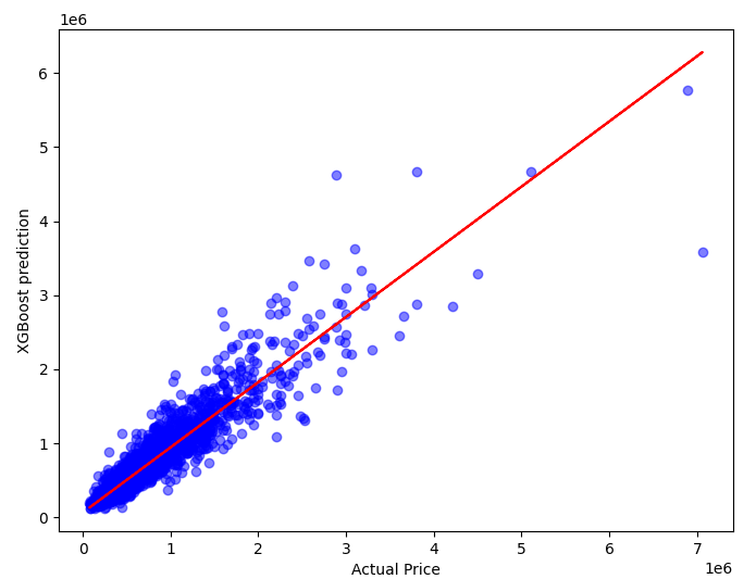
Figure 12. Four methods fit degree (Original)

While running the RF model, LR model and XGBoost model (ANN model generally not gives the importance of different features), we conducted an assessment of feature importance within our dataset. We used the coefficients trained by polynomial linear regression as the feature importance; RF-feature_importances_ and feature_importance were used to obtain the contribution degree of the feature value in the RF and XGBoost to perform feature ranking as the importance of the feature. The result of the feature importance comparison shows below (Table 3).

Table 3. Feature Importance

Leveraging these results, we computed an aggregate ranking of feature importance by assigning weights based on the accuracy of each algorithm. As displayed in Figure 13 below, our analysis reveals that the three most influential features affecting house prices in our dataset are in decreasing order of significance: "lat", "waterfront" and the "grade" of the house.

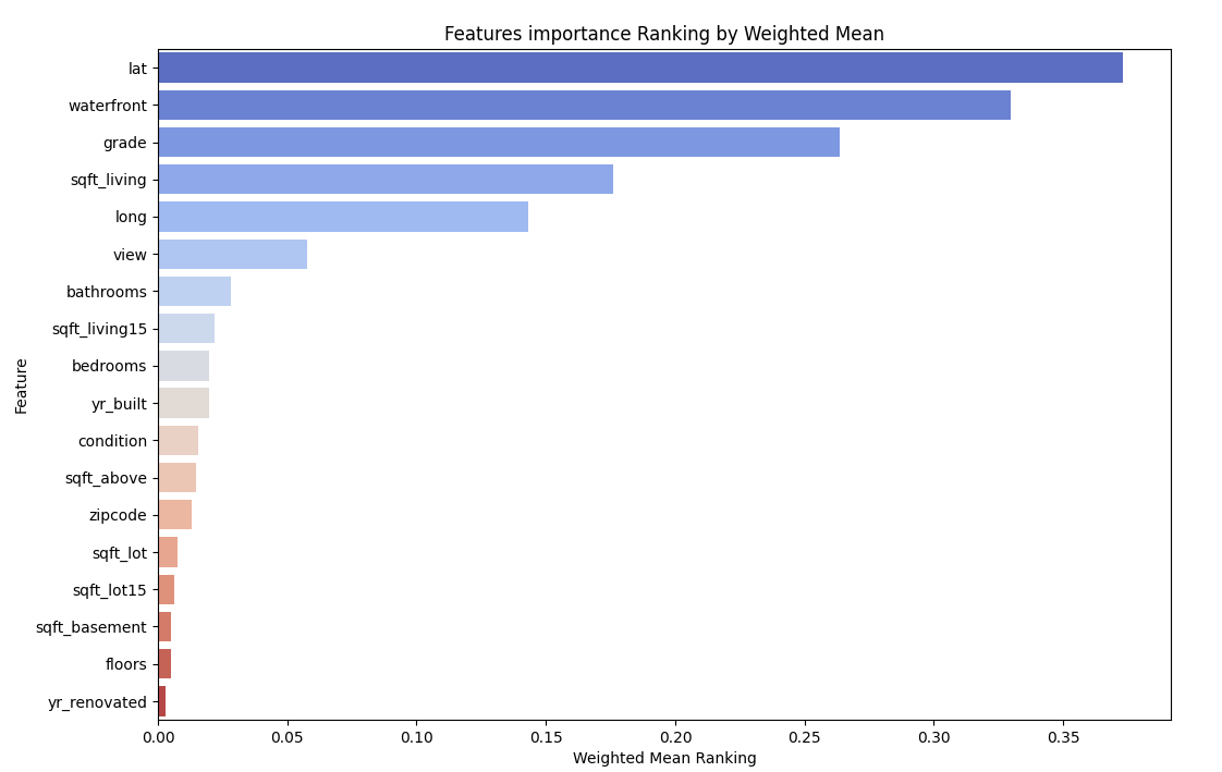
Figure 13. Overall feature ranking (Original)

5. Conclusion

This article examines three different house price prediction models and compares their accuracy. They are linear regression, random forest and network neural. This article explores the impact of each feature on price at same time.

In the experiment, we can see that XGBoost has the highest accuracy, linear regression has the lowest. Therefore, for predicting house prices, considering accuracy, the XGBoost method would be more suitable. In comparison with neural networks, random forests and XGBoost although linear regression has the lowest accuracy, its accuracy is relatively close to the other three methods. Considering that the linear regression method is relatively simple and straightforward, when time is limited and accuracy requirements are not so high, the linear regression method will be an option. More research is needed in this part.

Regarding the importance of features, we can see that the three most influential features affecting house prices in our dataset are lat, waterfront and grade in the experiment. In other words, for the houses we choose, their latitude, waterfront condition and house grade can most affect their prices. This result may hold true for other houses and be helpful in their price predictions. However, more research is needed to confirm this.

Future research should focus on the comparison of the time and space complexity of random forest and linear regression and the impact of the features of houses in other areas on their prices.

References

[1]. Maslow, A. H. (1943). A theory of human motivation. Psychological Review, 50 (4), 370-96.
[2]. “King County, Washington”, wikipedia, 31 October 2023, https://en.wikipedia.org/wiki/King_County,_Washington
[3]. House Sales in King County, USA, https://www.kaggle.com/datasets/harlfoxem/housesalesprediction/data
[4]. Visualization-on-a-Map https://www.kaggle.com/code/chrisbronner/regression-r2-0-82-and-map-visualization#3.
[5]. N. N. Ghosalkar and S. N. Dhage, "Real Estate Value Prediction Using Linear Regression," 2018 Fourth International Conference on Computing Communication Control and Automation (ICCUBEA), Pune, India, 2018, pp. 1-5, doi:10.1109/ICCUBEA.2018.8697639
[6]. Breiman L. Random Forests. SpringerLink. https://doi.org/10.1023/A:1010933404324 (accessed September 11, 2019).
[7]. Raschka S, Mirjalili V. Python machine learning: Machine learning and deep learning with Python, scikit-learn, and TensorFlow. 2nd ed. Birmingham: Packt Publishing; 2017.
[8]. Cireşan, D.C.; Meier, U.; Gambardella, L.M.; Schmidhuber, J. Deep, big, simple neural nets for handwritten digit recognition. Neural Comput. 2010, 22, 3207–3220.
[9]. T. Chen, C. Guestrin XGBoost: A scalable tree boosting system, Association for Computing Machinery (2016), pp. 785-794
[10]. W. Dong, Y. Huang, B. Lehane, G. Ma XGBoost algorithm-based prediction of concrete electrical resistivity for structural health monitoring and Automation in Construction, 114 (2020), p. 103155
Cite this article
Li,C. (2024). House price prediction using machine learning. Applied and Computational Engineering,53,225-237.
Data availability
The datasets used and/or analyzed during the current study will be available from the authors upon reasonable request.
Disclaimer/Publisher's Note
The statements, opinions and data contained in all publications are solely those of the individual author(s) and contributor(s) and not of EWA Publishing and/or the editor(s). EWA Publishing and/or the editor(s) disclaim responsibility for any injury to people or property resulting from any ideas, methods, instructions or products referred to in the content.
About volume
Volume title: Proceedings of the 4th International Conference on Signal Processing and Machine Learning
© 2024 by the author(s). Licensee EWA Publishing, Oxford, UK. This article is an open access article distributed under the terms and
conditions of the Creative Commons Attribution (CC BY) license. Authors who
publish this series agree to the following terms:
1. Authors retain copyright and grant the series right of first publication with the work simultaneously licensed under a Creative Commons
Attribution License that allows others to share the work with an acknowledgment of the work's authorship and initial publication in this
series.
2. Authors are able to enter into separate, additional contractual arrangements for the non-exclusive distribution of the series's published
version of the work (e.g., post it to an institutional repository or publish it in a book), with an acknowledgment of its initial
publication in this series.
3. Authors are permitted and encouraged to post their work online (e.g., in institutional repositories or on their website) prior to and
during the submission process, as it can lead to productive exchanges, as well as earlier and greater citation of published work (See
Open access policy for details).