1.Introduction

Stocks represent a form of security that represents partial ownership in a company. When investors purchase stocks of a company, they become shareholders and have corresponding rights and interests. Stock price refers to the buying and selling price of stocks in the market, which is influenced by various factors including the company's financial condition, industry trends, macroeconomic conditions, and investor sentiment.

In our research, we focus on predicting the stock prices of large institutions using a variety of machine-learning approaches. These include the k-nearest neighbors algorithm (KNN), supporting vector machine (SVM), naïve Bayes, random forest, linear discriminant analysis, and quadratic discriminant analysis. Our objective is to determine the most effective method for predicting specific stock prices.

The thesis has been organized in the following way: chapter 2 gives a brief review of recent related research about predicting the stock market using machine learning methods, and comparing the performance of different methods. Chapter 3 describes our approaches in acquiring and preprocessing the data used for research. Chapter 4 demonstrates feature engineering on our initial features. The detailed experiment process and result is illustrated in chapter 5 and 6. Chapter 7 contains the conclusion and includes a discussion of the implication of the findings to future research.

2.Literature Review

The prediction of stock prices can provide investors with valuable information about risks and suggestions on trading actions to be taken. Researchers have taken lots of machine learning approaches including SVM, random forest, etc. to counter the chaos and fluctuations in stock prices. Their research has provided valuable insights for other researchers, by pointing out that selecting large-scale companies pursuing a promising endeavor could effectively mitigate the impact of stock market volatility on predictions.

Researchers have used machine learning methods in prediction different kinds of stocks. Shaikh et al. used LSTM to predict the prices of stocks of several solar energy companies, since solar energy will play a crucial role in an environmental-friendly future [1].

Many researches have compared the performance of various machine learning approaches in predicting stock prices. Khoa and Huynh compared SVM, ANN and logistic regression in their research, and found that accuracy of logistic regression model is 59%, accuracy of ANN model is 60%, while accuracy of SVM model is 92% [2]. Chhajer, Shah and Kshirsagar (2022) compared ANN, linear and non-linear SVM and LSTM in their research, and concluded that LSTM outperform ANN and SVM in terms of accuracy [3].

Hybrid models are worth further studying. Those models often outperform traditional and simple ones. Ilyas et al. researched on a hybrid model which also takes social media comments as data and has a hodrick-Prescott filter [4]. Their model improves the predicting accuracy and R-square of SVM models and random forest models. Mahmoodi, et al. combined SVM with metaheuristic algorithms in their study [5]. The performance is enhanced to varying degrees with different algorithms.

Researchers using deep learning methods may make the model more complex, because the price of a stock is decided not only by its former prices, but also people’s expectations, comments and trading actions on this stock. In fact, knowing that investors’ actions and attitudes towards a certain stock may also influence its price, some researchers, such as Ilyas et al. and Koukaras, Nousi, and Tjortjis, used social media comments as data too [4,6]. Their model outperforms other models that only takes time-series prices of a stock as data.

3.Exploratory Data Analysis

The dataset used in this experiment is collected from Yahoo Finance, which in practice is achieved by importing the “yfinance” package in Python and outputting the raw data frame.

These stock price data are collected from companies in three different sectors: Internet, Security, and Banking companies in this experiment.

The raw data contains five indicators: the day's opening price, the day's highest price, the day's lowest price, the day's closing price and the day's trading volume. In this study, the closing price is considered as the response variable. Several missing values in the raw data, along with other data on the same trading day, are removed.

In this research, the time span of data used has yet to be unified in this experiment since different companies have different listing times. If the analysis periods are coerced to unified, it may result in some inaccuracies in the later analysis. Therefore, this research chose to include all companies from listing to 2023-09-07~2023-09-11 to minimize inaccuracies.

3.1.Data Standardization and Normalization

Data used in this project went through data standardization and normalization as follows for the different models fitted in this experiment. In the formula below,\( X \)is the raw data,\( μ \)is the mean value of the data set,\( σ \)is the standard deviation of the data set. In practice, two Python functions, StandardScaler and MinMaxScaler in Scikit-learn package are applied for these operations.

\( {X_{Standardized}}= \frac{X-μ}{σ} \)(1)

\(X_{\text{Normalized}} = \frac{X - X_{\min}}{X_{\max} - X_{\min}} \)(2)

3.2.Visualization & Analysis of Volume and Closing price

In our analysis, we scaled the 'Volume' variable by dividing it by a factor of 1e7, primarily to avoid numerical overflow issues during computation. This scaling doesn’t impact the computed correlation coefficient between 'Volume' and 'Close' price, as it preserves the relative distances and rankings among the original data points. The correlation coefficient remains constant because it is derived from the relative positioning of the data points, not their specific numerical values.

Hence, the calculated correlation coefficient after scaling the 'Volume' variable is identical to the one that would have been obtained without scaling, ensuring the validity of our correlation analysis results.

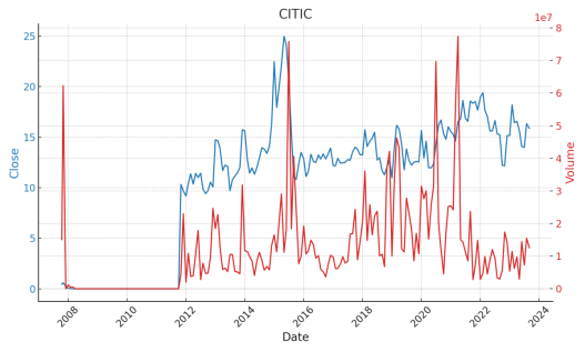
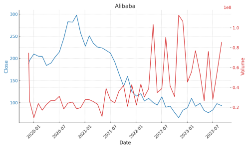
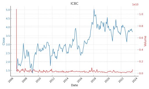
Figure 1. The 'Close' stock prices and 'Volume' of trades

As shown in the Figure 1:

CITIC Securities (CITIC):

•Trend: From 2008 to 2011, both the closing price and the trading volume of CITIC Securities remained almost constant, manifesting as a flat line. However, in subsequent years, there was a noticeable upward trend in both the closing price and trading volume.

•Volatility: Starting from 2012, the stock price and trading volume of CITIC Securities exhibited evident volatility, indicating increased market participation and dynamics.

•Key Observations: In recent times, while there have been prominent peaks in trading volume, the closing price appears to remain relatively stable.

Alibaba:

•Trend: From its initial public listing, Alibaba's stock price showed an upward trajectory, with the trading volume peaking during specific periods.

•Volatility: Compared to CITIC Securities, Alibaba's stock price and trading volume displayed greater fluctuations throughout, especially in certain time intervals.

•Key Observations: While there are periods of peak trading volumes, they don't always coincide with significant shifts in the stock price.

ICBC:

•Trend: On the whole, both the stock price and trading volume of ICBC remained relatively stable, without any pronounced long-term ascent or descent.

•Volatility: The trading volume for ICBC showed sporadic fluctuations at certain times, but these did not seem to result in substantial changes in the stock price.

•Key Observations: ICBC's stock appears to be comparatively resilient, without wide-ranging alterations in price and trading volume.

From the analysis, we can conclude the following:

Internet-related companies, owing to their emergent nature, exhibit greater volatility compared to the other two types of stocks analyzed. Furthermore, there appears to be a positive correlation between stock price and trading volume, signifying a tendency among traders to prefer purchasing such stocks when the prices are ascending. Such a positive correlation could be attributed to the high-growth potential perceived in Internet-related sectors, prompting investors to buy in anticipation of future price increases.

Securities-related stocks exhibit a contrasting behavior. Investors seem to adopt a contrarian approach, preferring to buy these stocks when prices decline, implying a relatively negative correlation between stock price and trading volume. This behavior might be driven by the belief that the securities sector, being relatively traditional, offers value-buying opportunities during market downturns, allowing investors to buy stocks at lower prices with the expectation of a rebound.

Bank stocks, particularly those with state ownership like ICBC, also exhibit a negative correlation; their fluctuations are relatively minimal, rendering them more stable than the other two stock categories. The observed stability in bank stocks could be attributed to their state-owned nature, which often assures investors of a certain level of security and resilience against market volatility, making them a preferred choice for risk-averse investors seeking consistent returns.

Additionally, from 2008 to 2011, the unusual trends in CITIC Securities stocks are believed to have stemmed from the significant effects of the global financial crisis, which heavily impacted stock markets. At the same time, ICBC's stability is linked to its state ownership, which probably buffered it against market fluctuations, ensuring resilience during financial upheavals.

4.Feature Engineering

There are copious predictors extant regarding stock price prediction. Regarding the choice of pertinent predictors, Patel et al. provided valuable insight into what predictors proved efficacious and assistive in fitting classification models [7]. The following predictors shown in Table 1 are produced and adapted from the work of these authors.

Moving averages smoothen time-series data to highlight long-term trends and reduce short-term noise, aiding in trend identification, and serving as potential support or resistance levels in technical analysis.

The weighted 10-day moving average (WMA) prioritizes recent data in time-series analysis, offering a more responsive view of market trends and effectively reducing short-term noise. It enhances machine learning stock prediction models by capturing time-dependent data structures.

"Momentum" is a technical analysis tool that gauges stock price trends. Positive values suggest potential upward trends, while negative values hint at downtrends. It measures historical price fluctuations, and extreme values might indicate potential trend reversals.

The Stochastic K% is a momentum oscillator assessing a security's current closing price relative to its high-low range over a set period. It detects potential overbought or oversold conditions, suggesting trend reversals or continuations. Its interactions with D% offer trading signals, while its shifts provide momentum insights and divergence detection for early price reversal indications.

Table 1. 9 features used to train the model

The Stochastic Oscillator, especially Stochastic D%, indicates overbought or oversold markets. D% smooths Stochastic K% to reduce noise. Values above 80 suggest overbought and below 20 indicate oversold conditions. Crossovers can signal trend changes.

The Relative Strength Index (RSI) is a 10-day momentum oscillator analyzing the magnitude of recent price changes to gauge overbought or oversold market conditions. Key indicators include: crossing the 50 level to signal bullish or bearish trends, confirming momentum by aligning with price highs or lows, and detecting divergences with price, which can presage potential reversals.

The Moving Average Convergence Divergence (MACD) is a momentum indicator comparing two moving averages of a security's price. Key signals include:

1.Signal line crossovers, indicating bullish or bearish trends.

2.Movements around the zero line, suggesting upward or downward momentum.

3.Divergences between price and MACD, hinting at potential price reversals.

The A/D Oscillator measures the link between an asset's price and volume, differentiating accumulation from distribution. Ranging between -1 and 1, positive values show accumulation, negative ones signal distribution, and zero means balance. Differences between the A/D and price trends can hint at market sentiment shifts.

The Commodity Channel Index (CCI) is an indicator used to spot cyclical turns in commodities by measuring the deviation between a security's current and average price change. Key insights from CCI include:

1.Identifying overbought (>+100) or oversold (<-100) conditions.

2.Gauging bullish or bearish sentiment with zero-line crossovers.

3.Detecting divergences between price and CCI for potential price movements.

4.Confirming market trends based on CCI's direction.

Table 1 shows the formula of the 9 features. In Table 1, Cₜ is the closing price, LL_t and HHₜ implies lowest low and highest high in the last t days, respective.

5.Experiment settings

5.1.Preprocessing

5.1.1.Data scaling. Min-Max scaling technique and Z-score normalization technique are applied to scale the numerical variables.

5.1.2.Data Partitioning for training data and testing data. The dataset is divided into two distinct subsets: a training set (X_train and y_train) and a testing set (X_test and y_test). The training set is utilized for model training, while the testing set is reserved for the evaluation of model performance. In this case, a 20% threshold is employed for the testing data.

5.1.3.PCA Dimensionality Reduction and Cross Validation Feature Selection. Applying Principle Component Analysis to reduce the dimensionality of dataset. The PCA process identifies the top 9 principal components, which are linear combinations of the original features capturing the maximum variance in the data. Following the initial PCA, we conduct an analysis of the contribution of each principal component to the overall variance of the data.

This contribution analysis, visualized as an explained variance ratio curve, displays the proportion of total variance explained by each principal component.

Instead of dimensionality reduction, a hand-made function emulating cross validation method is also written to select features. First is to split training data to the new training and testing data set analogous to the method of k-fold cross validation. The function then exhausts all combinations of feature to fit models and compute the accuracy of prediction to select the best combination of features to fit model. The pseudocode is given below:

Algorithm 1: Feature selection algorithm based on cross validation method

Input: model: model name,

Input: train: new training data produced by cross validation method,

Input: test: new test data produced by cross validation method,

Input: train_target: the response variable of the new training data,

Input: test_target: the response variable of the new testing data

feature <- matrix(NA, nrow=1+ncol(train), ncol = ncol(train)) ## Create result matrix

## Combining training data with response variable to prepare for fitting models

data.fit<-data.frame(train,Target=train_target)

for i in 1 to ncol(train) do

df <- combn(names(train), i) ## Obtain all combinations of features

temp_accu <- rep(NA, ncol(df)) ## Create list object to store prediction accuracy later

for j in 1 to ncol(df) do

## Combining using function “as.formula” and “paste” to massively create formula object to prepare for fitting model

f <- as.formula do

paste do

"Target~",

paste(names(train[df[,j]]),collapse= "+")

end do

end do

## Plug in formula object and data frame object to fit model.

fit <- model(f, data.fit)

## Since the grammars differ at prediction phase for different models, using “tryCatch” structure to exhaust all grammars.

pred <- tryCatch try

predict(fit, test)

if wrong, retry

predict(fit, test, type = "prob")

end try

table.pred <- tryCatch try

table(Actua=test_target, Predicted = pred)

if wrong, retry

tryCatch try

table(Actual = test_target, Predicted = pred$class)

if wrong, retry

table(Actual = test_target,

Predicted = cut(pred, breaks = c(-Inf, 0.5, Inf), labels = c(0,1)))

end try

end try

## Compute prediction accuracy and store it in the list object created before

rate<-sum(

diag(table.pred))/ length(test_target)

temp_accu[j] = rate

end for

## Plug in the accuracy and corresponding feature combination into the feature matrix

feature[1,i] = round(max(temp_accu),4)

feature[2:(i+1),i]= df[,which.max(temp_accu)]

end for

## Output the data frame object which stores selected features

data.frame(feature)

5.1.4.Data input for modelling. Following the dimensionality reduction achieved by PCA to a 2D feature space, and the feature selection process by cross validation method, the final datasets are produced respectively regarding two data processing methods. For PCA processed dataset, the predictors are the PCs produced, and for CV processed dataset, predictors are selected features. The response variables are both the dichotomy factor variables representing the increase or decrease of stock prices. It is substantiated that the selected features are more effective in prediction of testing data.

5.2.Model Fitting

5.2.1.K-Nearest Neighbors (KNN). Parameter tuning by Cross-Validation (TimeSeriesSplit)

Function of Time Series Cross-Validation (TimeSeriesSplit) is applied to partition the dataset for the purpose of cross-validation. This technique partitions the dataset into multiple non-overlapping subsets, or "folds," facilitating repeated model training and testing. By navigating divers subsets of the data, it helped to tune parameters of the KNN model.

Parameter tuning by Grid Search

This model relies on proximity-based classification, wherein data points are classified based on their proximity to the nearest neighbors. A grid search procedure (GridSearchCV) is executed to explore various parameter combinations and identify the optimal configuration for the K-Nearest Neighbors classifier.

Model Fitting:

Utilizing the optimal K value determined through the grid search and Cross-Validation, a K-Nearest Neighbors classifier model is fitted on training dataset. Then the model is available to make predictions based on test dataset.

5.2.2.Support Vector Machines (SVM)

•Basic SVM Model Setup: Initialized SVM with initial hyper parameters including the penalty parameter C and a linear kernel.

•Bayesian Optimization for SVM:

Setup: Bayesian optimization techniques are applied to discover the optimal configuration of SVM model hyper parameters. An objective function (svm_cv) is defined for optimization, which accepts C and gamma as inputs and employs cross-validation to compute the model's performance score.

Search Space: Defined the hyper parameter search space, focusing on C and gamma.

Optimization Process: Executed Bayesian optimization to discover the best hyper parameters.

Results: Displayed the optimal hyper parameters identified.

•Grid Search for SVM:

Setup: Used GridSearchCV to systematically explore optimal SVM hyper parameters.

Parameter Grid: Set the grid for hyper parameters, including C, kernel type, degree, and gamma.

GridSearchCV Execution: Conducted grid search, testing different hyper parameter combinations using cross-validation.

Results: Showed the best hyper parameters and the corresponding best estimator.

•Model Fitting and Predictions:

Fitted SVM models using hyper parameters from Bayesian Optimization and Grid Search.

Made test data predictions with both models, resulting in two classification outcomes.

5.2.3.Naïve Bayes. Prior probability setting

The prior probability is supposed to differ by different companies. Hence it is set according to the proportion of increase in the training dataset.

Laplace Smoothing Value Setting

In other multi-classification tasks, the Laplace smoothing method is specified in order to evade the potential problem of “0-probability” in certain class. However, for this dichotomy classification, there is no need to apply Laplace smoothing method. Therefore, the value is set to 0.

The rest part is fitting the naïve Bayes model on training data using selected features and PCs and make prediction on test data.

5.2.4.Linear/Quadratic Discriminant Analysis (LDA, QDA) and Logistic Regression. Given that features are selected and PCs also produced, there is no other model-specific parameters need to be tuned. Then, the processes at model fitting phase for these three models are the same. Using selected features and dimensionally reduced PCs, three models are fitted on training data and in preparation to make predictions on testing data.

5.3.Experiment Setting for Random Forests

Owing to the unique characteristics of the random forest, it has its own data processing and model fitting procedures. We will now discuss the experimental settings for the random forest.

5.3.1.Data processing. Delete Outlier: In the processed data, some data have missing values, maximum values, minimum values, etc. While ensuring the amount of data, the impact of these values on model training can be resolved by taking measures to delete rows containing these values. Unlike other models, since the random forest algorithm is built on the basis of a tree model, the scale of the data does not affect the model. Therefore, for random forest models, there is no need to normalize the data set.

Partition the Data Set: For all data sets, we randomly selected 80% of the data as the training set for model training, and retained 20% of the data as the prediction set to detect the effect of the model.

Use cross validation set for parameter tuning: Each classification tree model in the random forest needs parameter tuning based on different data. The key parameter in the random forest model is ‘mtry’,which represents the number of features randomly selected each time the classification tree algorithm is performed. Through the method of 5-fold cross validation set for random forest, we can choose the most appropriate ‘mtry’ value for different data. A 5-fold validation set is a dataset divided into five subsets of equal size. It is commonly used in machine learning to evaluate the performance of a model. The model is trained on four subsets and tested on the remaining one, with this process repeated five times to ensure robustness in the evaluation. The selection results are as follows in Table 2, 3, 4:

Table 2. Random Forest parameter values for securities companies

Table 3. Random Forest parameter values for network companies

Table 4. Random Forest parameter values for banks

Substitute the adjusted parameters into the random forest training model to get the optimal fitting result.

5.3.2.Model Fitting. The parameter fitting for Random Forest:In the random forest algorithm, for different data, we substitute the optimal mtry parameters calculated through the 5-fold cross validation set into the model, and set the subtrees in all random forest models to 1000 for model fitting training. The advantage of setting the subtree to 1000 is to ensure a sufficient number of subtrees, making the classification ensemble algorithm more stable and accurate in the final voting. For other parameters, we use the default parameters in the R language random Forest package

Model training: A pseudocode about the process of random forest algorithm is as follows:

def random_forest (D, T, max_depth, max_features):

trees = []

for t in range(T):

features=random.sample(D.features, max_features)

subset = random.sample(D, len(D))

tree=build_decision_tree(subset, max_depth, features)

trees.append(tree)

return trees

def build_decision_tree (D, max_depth, features):

if all_samples_have_same_label(D):

return LeafNode(D[0].label)

if len(features) == 0 or max_depth == 0:

label = majority_label(D)

return LeafNode(label)

best_feature=select_best_feature(D, features)

subsets = split_dataset(D, best_feature)

left_subtree=build_decision_tree(subsets[0], max_depth - 1, features)

right_subtree=build_decision_tree(subsets[1], max_depth - 1, features)

node=DecisionNode(best_feature, left_subtree, right_subtree)

return node

In random forest fitting process, the model is trained on the data to identify the patterns of all 1000 subtrees. The basis for dividing the tree is the Gini coefficient. The Gini coefficient can reflect the purity of a collection. The smaller the Gini coefficient, the higher the purity. Each time the classification tree is divided, it will select the dividing method that can minimize the Gini coefficient sum of all divided sets. Finally, combining the final votes of all subtrees, we can make predictions about the data.

5.4.Model Evaluation

5.4.1.Probability Prediction. We used the KNN classifier to predict the probability of a stock belonging to the positive class based on its price.

5.4.2.ROC Curve. The ROC curve showcases the classifier's performance at different thresholds.

"ROC AUC" gives a single number summary of the curve. A higher ROC AUC indicates better performance.

It's plotted with FPR on the x-axis and TPR on the y-axis. A diagonal dashed line represents random guessing.

5.4.3.Confusion Matrix Visualization. This visual displays how many predictions our model got right and wrong, split into four categories: TN, FP, FN, and TP.

5.4.4.Classification Report. This report gives a snapshot of how well our KNN classifier is performing.

•Precision: Indicates the accuracy of the model's predictions for each class.

•Recall: Measures the model's ability to identify all instances of a specific class.

•F1-Score: Gives a balance between Precision and Recall, especially useful for imbalanced datasets.

•Support: Tells the number of samples in each class.

6.Result and Discussion

6.1.Result of Feature Analysis

To visualize the effect of different features have on different companies, the ROC curves displayed the prediction effects of all features on all companies. The value showed in the legends are the AUC (area under the curve) value of each curve.

Network Companies

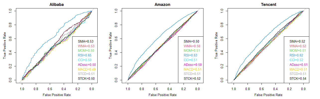
Figure 2. Features curve for network companies

Banks

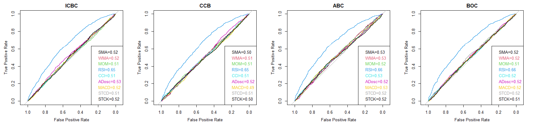
Figure 3. Features curve for banks

Securities Companies

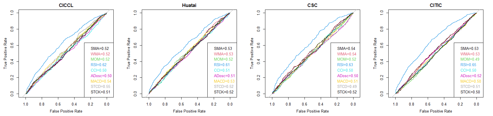
Figure 4. Features curve for securities companies

As Figure 2, 3, 4 all shown, “RSI” demonstrated to be the most effective feature in classifying observations in all three kinds of companies. Apart from this, other features behaved quite uniformly that all have no discernible effects on binary classification.

The feature selection algorithm played an instrumental role in filtering out the most powerful combinations of features. Exemplified by LDA\QDA, Naïve Bayes and Logistic regression, Figure 5, 6, 7 histograms display the frequency of each feature being chosen.

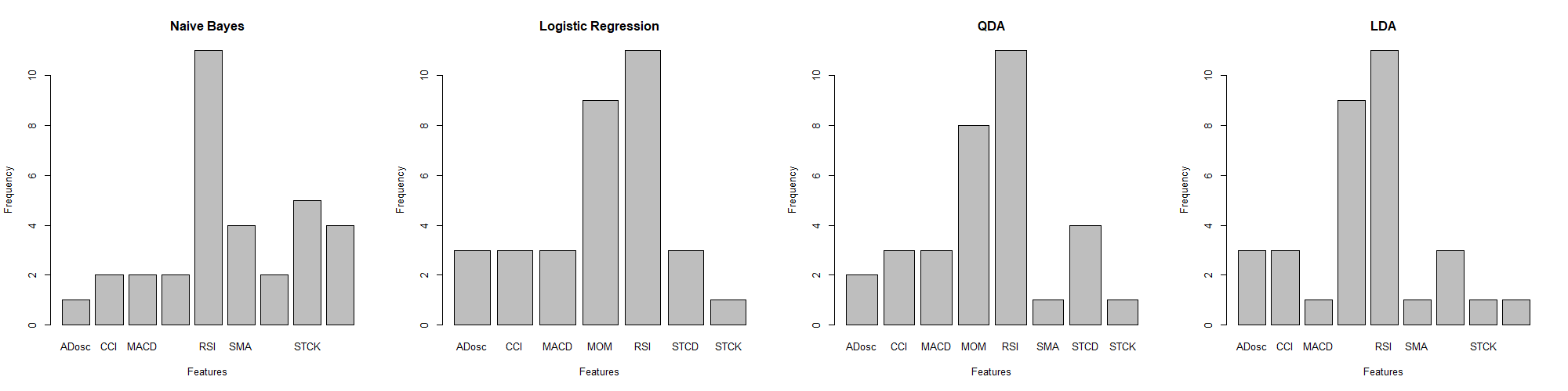
Figure 5. Models with 3 Features

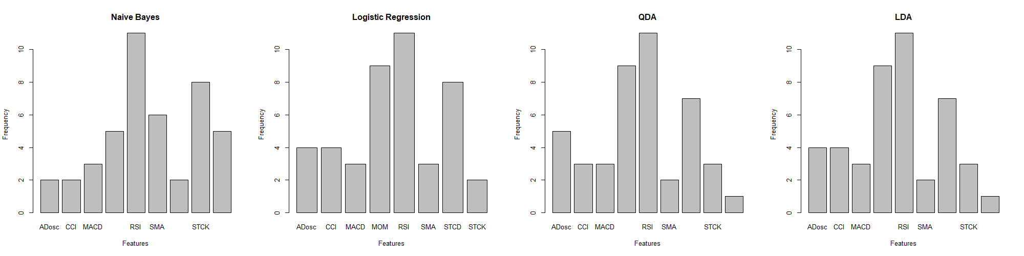
Figure 6. Models with 4 Features

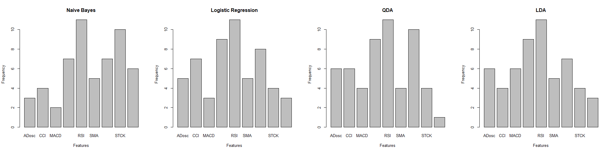
Figure 7. Models with 5 Features

As discussed before, RSI as the most effective feature, is selected most frequently in three figures. Especially in Figure 5, when features selected at a relatively scarce level, the RSI is predominantly selected among all features. In Figure 5, it can be also notice that MOM has the second large predictive effect across three situations on all companies. In Figure 6, when 4 features are applied, STCK is also selected at a relatively high frequency. Finally in Figure 7, when 5 features are adopted, another high predictive effect can be seen on STCD.

6.2.Result of Model Analysis

6.2.1.For Technology Companies (Alibaba, Amazon, Tencent)

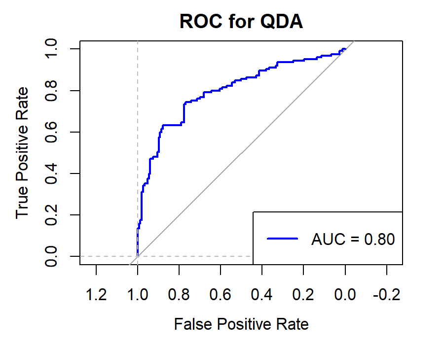
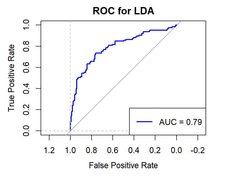
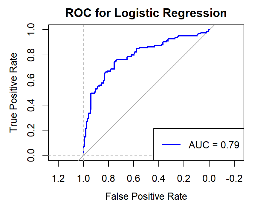
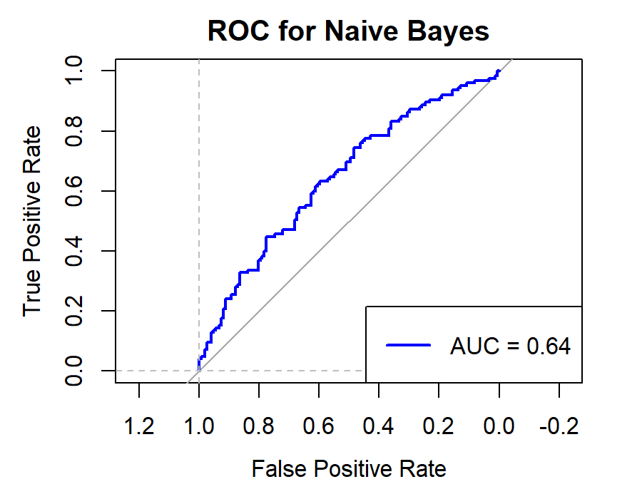
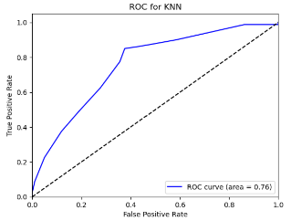
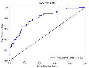
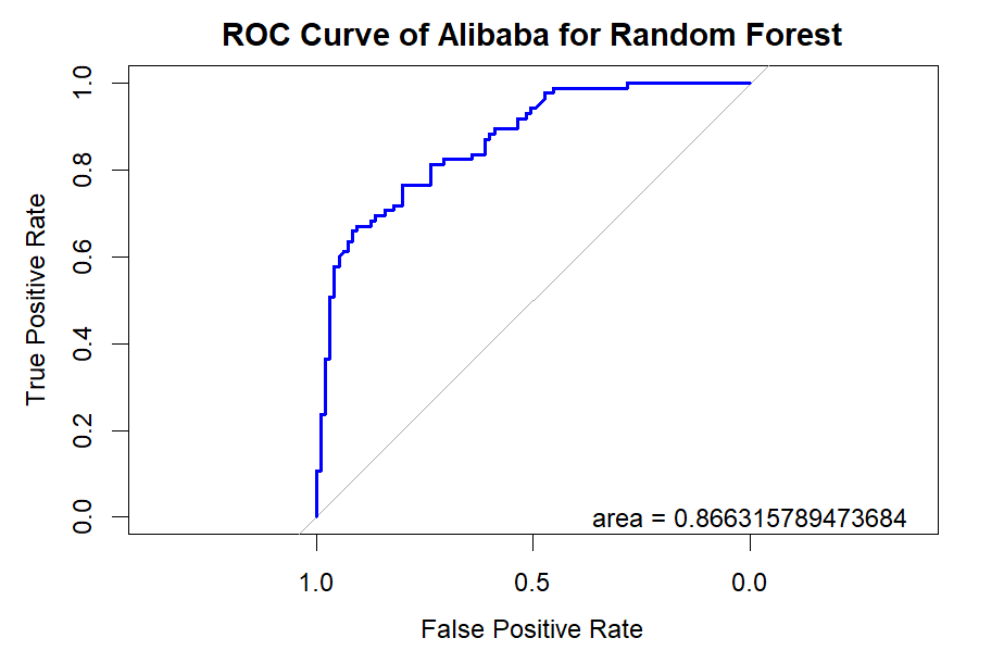
Figure 8. Roc curve comparison of Technology Company (Alibaba)

Figure 8 displays the Roc curve about the Alibaba(technology company), from which, we can draw the conclusion as following.

Summary for Technology Companies:

•Random Forest (RF) remains the top choice for its consistently high Accuracy, Precision, Recall, and F1-score.

•Logistic Regression (LR) and Quadratic Discriminant Analysis (QDA) also prove effective, particularly in terms of Accuracy and Precision.

•Other models like Linear Discriminant Analysis (LDA), Support Vector Machine (SVM), and K-Nearest Neighbors (KNN) exhibit reasonable performance but generally fall short of the top three.

•Naïve Bayes (NB) appears less suitable for this type of data.

6.2.2.For Banking Companies (ICBC, CCB, ABC, BOC)

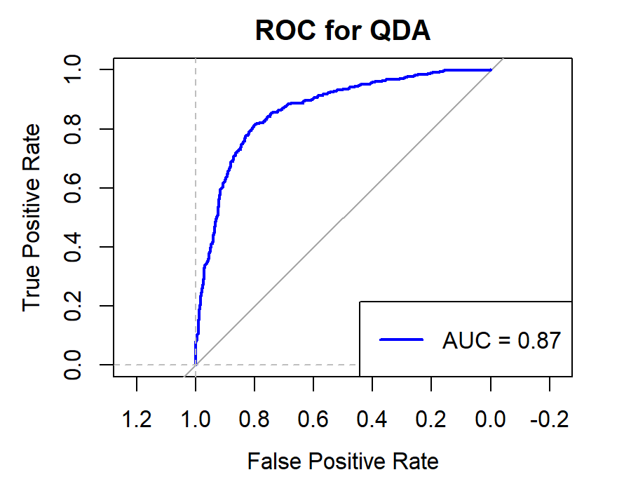
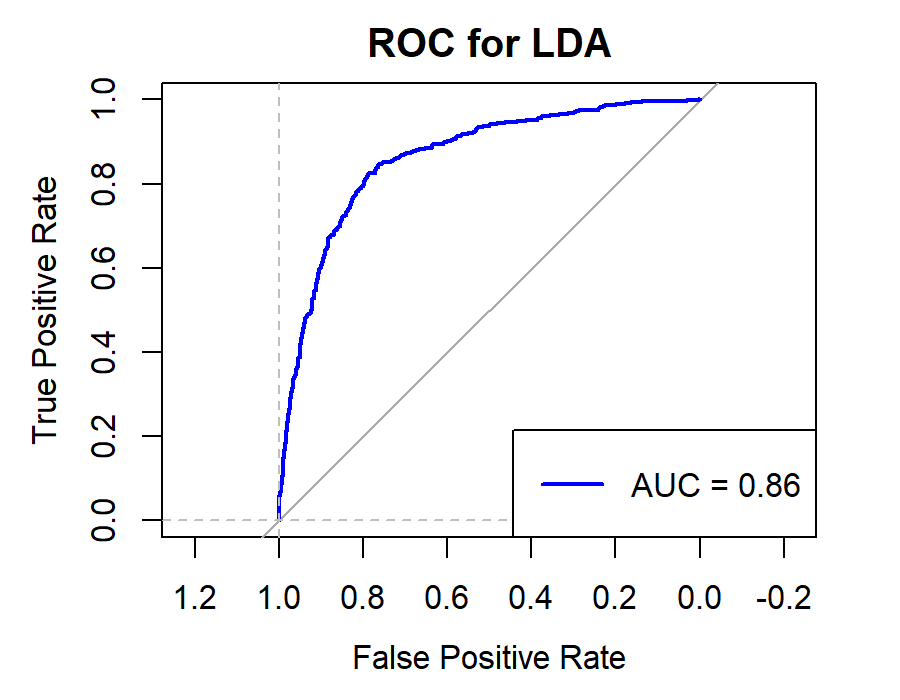
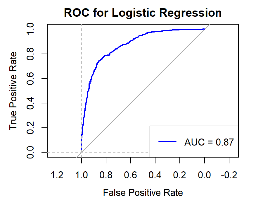
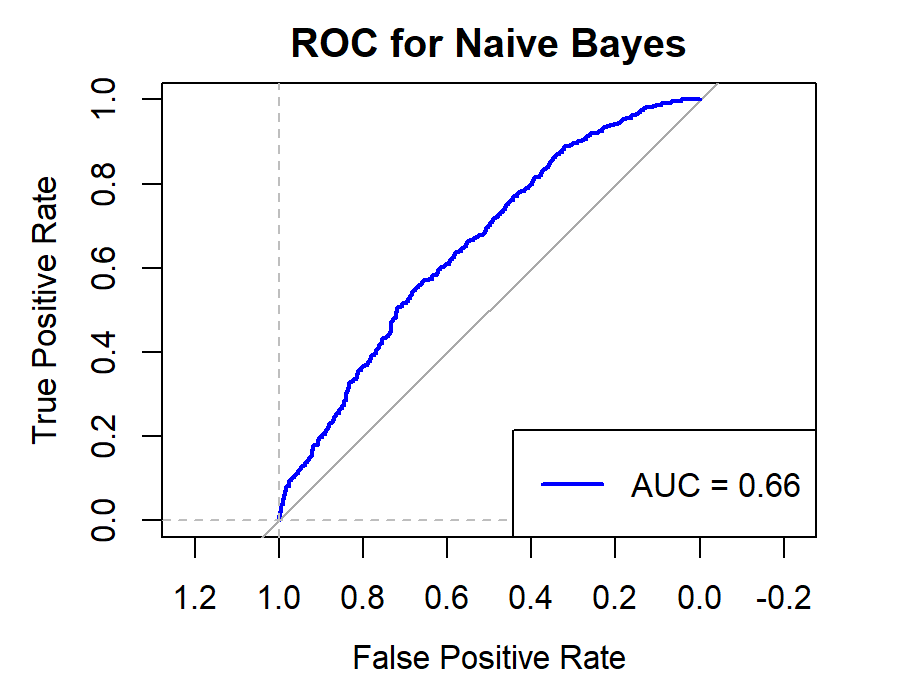
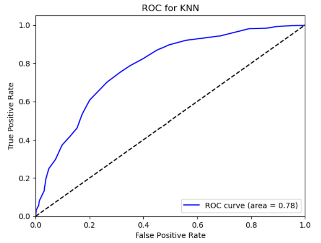
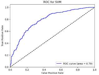
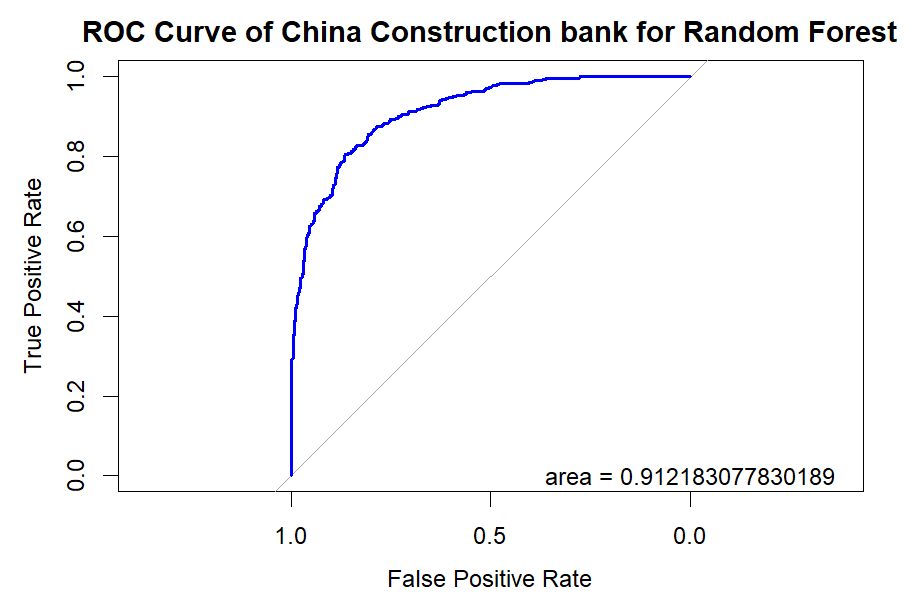
Figure 9. Roc curve comparison of Bank (CCB)

Figure 9 showcases the Roc curve about the China Construction Bank(Banking Company), from which, we can draw the conclusion as follows.

Summary for Banking Companies:

•For banking companies, both Random Forest (RF) and Logistic Regression (LR) are highly effective models, with RF having a slight edge in some cases.

•K-Nearest Neighbors (KNN) is the least effective model, possibly due to the high correlation between features or noise in the data.

•Support Vector Machine (SVM), Naïve Bayes (NB), and Linear Discriminant Analysis (LDA) perform moderately, with SVM and NB being competitive in some metrics.

6.2.3.For Securities Companies (CICCL, Huatai, CSC, CITIC)

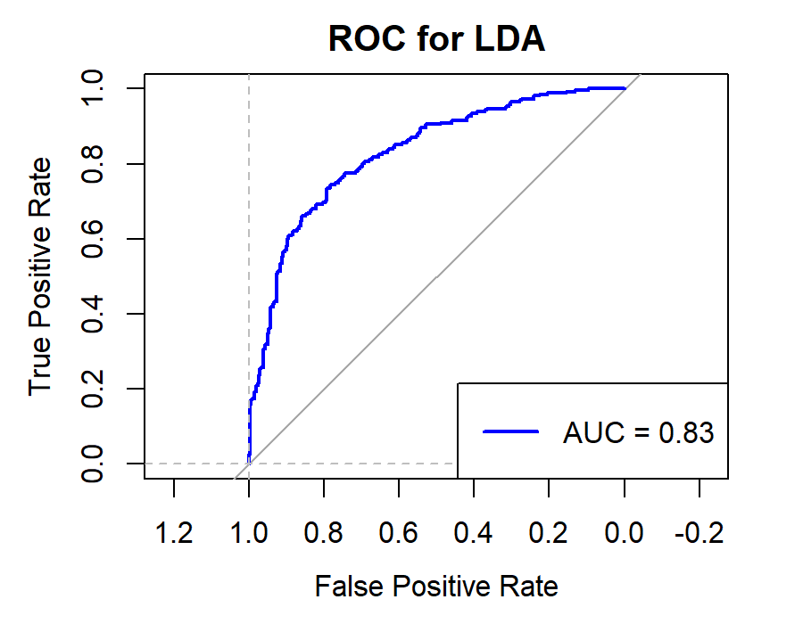
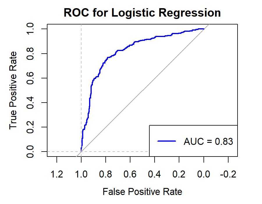
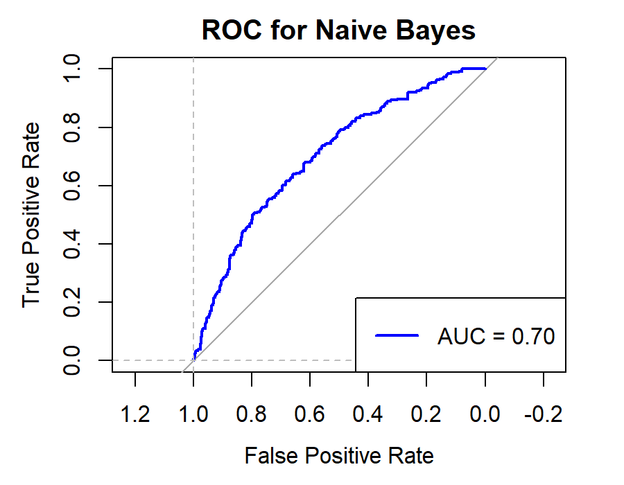
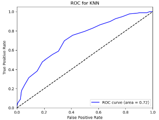
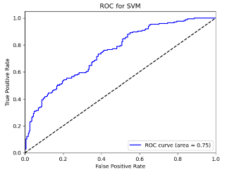
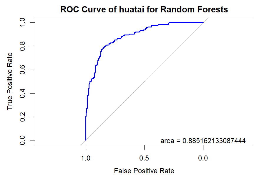
Figure 10. Roc curve comparison of Securities Company (Huatai)

Figure 10 showcases the Roc curve about Huatai(Security Company), from which, we can draw the conclusion as following.

Summary for Securities Companies:

•Random Forest (RF) remains the top choice, particularly for its high Accuracy and Precision.

•Linear Discriminant Analysis (LDA) and Logistic Regression (LR) also prove effective, especially in terms of Accuracy and Precision.

•K-Nearest Neighbors (KNN) underperforms for securities companies, underscoring the importance of model selection.

•Naïve Bayes (NB) and Quadratic Discriminant Analysis (QDA) offer moderate performance but generally fall short of RF, LR, and LDA.

6.2.4.For All Companies. In summary, different models exhibit varying performance across different types of company data. The choice of the appropriate model should consider specific business requirements and data characteristics. However, Random Forest (RF) consistently stands out as a robust choice, delivering high Accuracy, Precision, Recall, and F1-score across various scenarios. Additionally, Logistic Regression (LR) and Linear Discriminant Analysis (LDA) are suitable for situations requiring simpler and interpretable models.

7.Conclusion

7.1.Summary

In summary, this research embarked with the objective of analyzing and predicting binary classifications of stock price movements, striving to identify the most well-rounded model for executing this task efficiently. The experiment compared seven machine learning models, which are: Naive Bayes, LDA, QDA, logistic regression, KNN, support vector machine, and random forests. To encompass a diverse and contrasting range of stocks, securities, banking, and technology sectors were meticulously chosen, each representing distinctive market dynamics and variations.

In order to better improve the prediction accuracy of each model, we selected 9 features selected from the paper "Predicting stock and stock price index movement using Trend Deterministic Data Preparation and machine learning techniques" as explanatory variables and substituted some or all them into these seven models. Experimental results prove that these nine features can significantly improve the prediction accuracy of the model.

In the models training process, except for Amazon, whose data comes from the PNK stock market, the stock data of other companies come from the HKG stock market. Selecting data from the same stock market can reduce the interference of external factors on stock data. For all data, we performed preprocessing operations such as deletion of missing values and regularization. We screened these 9 features using a hand-made function emulating cross validation method, and used the selected features in six other algorithms except random forests, which significantly improved the prediction accuracy.

For the prediction results of the model, we found that random forest achieved the best prediction effect. In addition, for the two-category prediction problem of price rise and fall in the stock market, the LDA, QDA and Logistic Regression are also good choices in such questions. K-Nearest Neighbors(KNN) and Support Vector Machine(SVM) generally underperform. The Naive Bayes algorithm is not suitable for binary classification problems.

7.2.Future Work

Although this research achieved some meaningful results, there are still some limitations and shortcomings that provide opportunities for further research in the future. In the following aspects, we propose some possible research directions and improvements:

Expanding the sample size: The sample size of this study was relatively small, which may have some impact on the reliability of the results, especially for the machine learning models which require large sample sizes of the data. Future research can further validate our findings by increasing the sample size.

Combine different models to improve prediction accuracy: This experiment used seven relatively single models to predict the rise and fall of stock prices. However, if different models can be combined organically, the prediction accuracy of the models may be improved to a higher level.

Select other features: In this experiment, the features we selected were generated based on the daily opening price, closing price, highest price and lowest price of the stock. We have not considered external factors such as people's expectations for the prospects of these industries, media opinions, and relevant government policies. Future research can further combine these factors to improve the prediction accuracy of the model.

Explore the prediction accuracy of these machine learning algorithms in stock markets in other industries: In this experiment, we only studied three industries: the Internet, banks and securities companies. In order to make our research more general, in future work we can further explore the stock markets of other industries, such as technology companies, heavy industry companies, etc.

Overall, this study provides some implications and directions for further research in the future. Through the above future work, we can further deepen our understanding of the research problem and provide more valuable suggestions and guidance for practical applications.

Acknowledgment

KeQian Liu and Ang Li contributed equally to this work and should be considered co-first authors.

Xinran Lin, Zhuobin Mao and Weiyang Zhang contributed equally to this work and should be considered co-second authors.

References

[1]. Shaikh, Z. A., Kraikin, A., Mikhaylov, A., & Pinter, G. (2022). Forecasting Stock Prices of Companies Producing Solar Panels Using Machine Learning Methods. Complexity (New York, N.Y.), 2022, 1–9. https://doi.org/10.1155/2022/9186265
[2]. Khoa, B. T., & Huynh, T. T. (2022). Forecasting stock price movement direction by machine learning algorithm. International Journal of Electrical and Computer Engineering (Malacca, Malacca), 12(6), 6625. https://doi.org/10.11591/ijece.v12i6.pp6625-6634
[3]. Chhajer, P., Shah, M., & Kshirsagar, A. (2022). The applications of artificial neural networks, support vector machines, and long–short term memory for stock market prediction. Decision Analytics Journal, 2, 100015. https://doi.org/10.1016/j.dajour.2021.100015
[4]. Ilyas, Q. M., Iqbal, K., Ijaz, S., Mehmood, A., & Bhatia, S. (2022). A Hybrid Model to Predict Stock Closing Price Using Novel Features and a Fully Modified Hodrick–Prescott Filter. Electronics (Basel), 11(21), 3588. https://doi.org/10.3390/electronics11213588
[5]. Mahmoodi, A., Hashemi, L., Jasemi, M., Mehraban, S., Laliberté, J., & Millar, R. C. (2023). A developed stock price forecasting model using support vector machine combined with metaheuristic algorithms. Opsearch, 60(1), 59–86. https://doi.org/10.1007/s12597-022-00608-x
[6]. Koukaras, P., Nousi, C., & Tjortjis, C. (2022). Stock Market Prediction Using Microblogging Sentiment Analysis and Machine Learning. Telecom (Basel), 3(2), 358–378. https://doi.org/10.3390/telecom3020019
[7]. Patel, J., Shah, S., Thakkar, P., & Kotecha, K. (2015). Predicting stock and stock price index movement using Trend Deterministic Data Preparation and machine learning techniques. Expert Systems with Applications, 42(1), 259–268. https://doi.org/10.1016/j.eswa.2014.07.040
Cite this article
Liu,K.;Li,A.;Lin,X.;Mao,Z.;Zhang,W. (2024). Empirical study on the performance of various machine learning models in predicting stock price movements as a binary classification task. Applied and Computational Engineering,55,129-144.
Data availability
The datasets used and/or analyzed during the current study will be available from the authors upon reasonable request.
Disclaimer/Publisher's Note
The statements, opinions and data contained in all publications are solely those of the individual author(s) and contributor(s) and not of EWA Publishing and/or the editor(s). EWA Publishing and/or the editor(s) disclaim responsibility for any injury to people or property resulting from any ideas, methods, instructions or products referred to in the content.
About volume
Volume title: Proceedings of the 4th International Conference on Signal Processing and Machine Learning
© 2024 by the author(s). Licensee EWA Publishing, Oxford, UK. This article is an open access article distributed under the terms and
conditions of the Creative Commons Attribution (CC BY) license. Authors who
publish this series agree to the following terms:
1. Authors retain copyright and grant the series right of first publication with the work simultaneously licensed under a Creative Commons
Attribution License that allows others to share the work with an acknowledgment of the work's authorship and initial publication in this
series.
2. Authors are able to enter into separate, additional contractual arrangements for the non-exclusive distribution of the series's published
version of the work (e.g., post it to an institutional repository or publish it in a book), with an acknowledgment of its initial
publication in this series.
3. Authors are permitted and encouraged to post their work online (e.g., in institutional repositories or on their website) prior to and
during the submission process, as it can lead to productive exchanges, as well as earlier and greater citation of published work (See
Open access policy for details).