1. Introduction

Based on decision trees, there are two combinatorial algorithms. Both of them can be used for classification, they are random forest and adaboost algorithm. The classification effect is generally much better, compared with the classical linear discrimen.

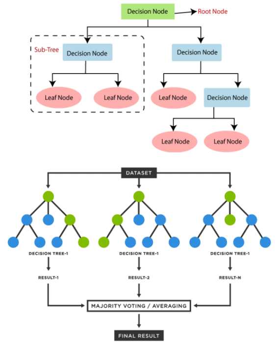
Figure 1. Diagram of decision trees and random forests

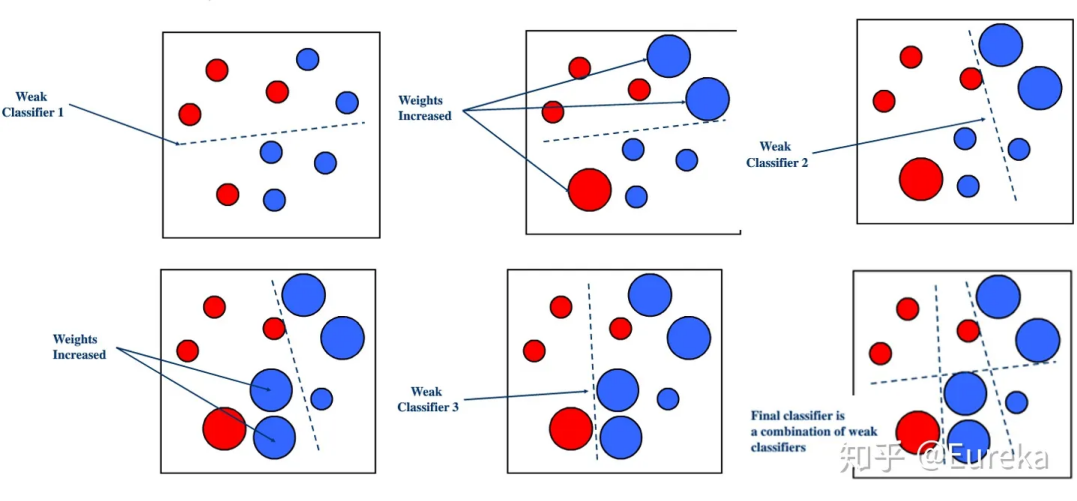
Figure 2. Diagram of Adaboost

Therefore, in this paper, we will discuss the characteristics of decision tree, random forest and adaboost algorithm in solving problems, and propose better selection schemes for different scenarios

2. Definition of Classification

2.1. definition

A classifier is a classification model built on existing data, which can associate data records in a database with specific categories for data prediction. The utilization of machine learning algorithms is aimed at enhancing efficiency and performance.

2.2. Construction and implementation of classifier

The construction and deployment of the classifier involve the following steps:

a. Sample selection: Choose positive and negative samples and divide them into training and testing sets.

b. Model implementation: Generating a classification model involves applying the classifier algorithm to the training set.

c. Prediction: Use the classification model to predict the labels of the test samples.

d. Evaluation: Calculate evaluation metrics based on the prediction results to assess the performance of the classification model.

2.3. Several basic classifiers

(1) Decision tree classifier: The decision tree utilizes a set of attributes to classify data, making a series of decisions based on the attribute set.

(2) Selection tree classifiers: Selection tree classifiers use similar techniques to decision tree classifiers to classify data.

(3) Evidence classifier: Classifies data by examining the likelihood of a particular outcome.

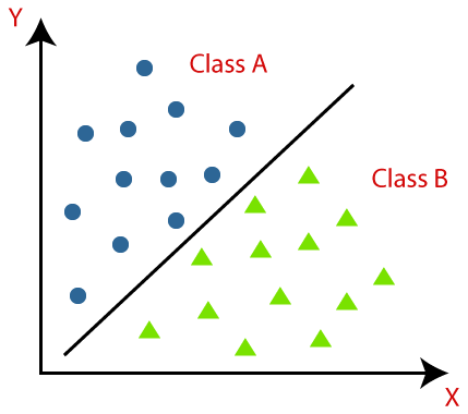
Figure 3. Schematic diagram of classifier

Our mainly work in the report.

In this research, our group aims to compare different ensemble learning methods for classification. Ensemble learning is an important area of machine learning that combines multiple models to improve overall predictive performance. The three algorithms we focus on are decision trees, random forests, and AdaBoost (adaptive boosting). Using standard datasets, we train and evaluate models using each technique. The evaluation metrics allow us to compare the accuracy, computational efficiency, and interpretability of the different methods. Our experiments show that random forests achieve the highest accuracy overall, while AdaBoost is the most efficient. Decision trees offer better interpretability than the ensemble methods. In conclusion, our work provides a comprehensive comparison of these popular ensemble learning techniques on a variety of criteria. Further research could explore ensembling deep neural networks or applying these methods to other domains. This study enhances understanding of the strengths and weaknesses of each approach to guide usage and future development.

In the following research, our group will.

The following research would cover the methodology of three classification algorithms - decision tree, random forest, and adaptive boost - for analysis on a heart disease dataset. The methodology section describes each algorithm. The decision tree algorithm recursively partitions the data space to construct a tree that models the classification. The random forest algorithm constructs an ensemble of decision trees trained on random subsets of features. The adaptive boost algorithm trains an ensemble of weak classifiers iteratively, adjusting sample weights to focus on misclassified instances.

The experiments section describes the heart disease dataset, comprising patient features like age, blood pressure, and presence of heart disease. Experimental settings and evaluation metrics are defined. The three algorithms are trained and tested using cross-validation.

3. Methodology

3.1. Algorithm 1 [decision tree]

3.1.1. Introduction. A decision tree is a classification algorithm that categorizes data items by asking a series of questions about their associated features. Each question is represented by a node, and internal nodes have child nodes corresponding to each possible answer. This hierarchical structure forms a tree-like representation. In its simplest form, the questions are yes-or-no queries, and each internal node has a "yes" child and a "no" child.

To classify an item, we traverse the decision tree starting from the topmost node, known as the root, and follow the path that aligns with the item's feature-based answers. Eventually, we reach a leaf node, which has no children, and assign the item to the class associated with that leaf.

In some variations of decision trees, the probability distribution over the classes is stored in each leaf node. This distribution estimates the conditional probability of an item belonging to a specific class, considering the path it took to reach the leaf. However, estimating unbiased probabilities can be challenging [1].

3.1.2. The Entropy of decision tree. Entropy is a concept derived from information theory and plays a crucial role in decision trees. In the context of decision trees, entropy is a measure of impurity or disorder within a dataset. It quantifies the level of uncertainty in the target variable and helps in determining the splitting criterion for each node in the tree. This measure helps decision trees find the most informative features to make effective decisions [2-3].

Entropy is widely used in decision tree algorithms, such as C4.5 and ID3, to evaluate the quality of a split. A decision tree starts with a root node representing the entire dataset. Entropy is calculated for this node, and then the dataset is split based on different attributes or features. The attribute with the highest information gain, which is determined by the reduction in entropy, becomes the splitting criteria for the current node. This process is recursively applied to build the decision tree until a predefined stopping criterion is met.

By minimizing the entropy at each step, decision trees aim to maximize information gain and create the most informative splits. Entropy helps in achieving a balance between exploration and exploitation of data, thus making decision trees more robust and accurate [4].

3.1.3. Decision Tree Algorithm. The decision tree algorithm is utilized to construct a predictive model based on the dataset. Given a set of input features and their associated target variable, the decision tree algorithm recursively splits the dataset based on the most informative attribute, creating decision nodes and leaf nodes. The decision nodes test the attribute value, and the leaf nodes represent the final prediction. The splitting process is determined by various splitting criteria, such as entropy, Gini index, or information gain.

3.1.4. Splitting Criterion. The splitting criterion measures the impurity or homogeneity of a node. Entropy and Gini index are commonly used splitting criteria. Entropy is defined mathematically as:

\( E(T)=-\sum p(c)×{log_{2}} \) p(c)

Let E(T) represent the entropy of a node, where p(c) denotes the fraction of instances belonging to class c, and the summation is carried out across all classes.

The Gini index is another splitting criterion defined mathematically as:

\( G(T)=1-\sum {p(c)^{2}} \)

The function E(T) calculates the entropy of a node, where p(c) represents the fraction of instances belonging to class c. The formula includes the summation of the entropy values across all classes.

Similarly, the function G(T) computes the Gini index of a node. It involves the proportion of instances (p(c)) belonging to class c, and the Gini index is calculated by summing the values over all classes.

3.1.5. Model Evaluation. Model evaluation is an essential stage in gauging the performance and efficacy of decision trees. It involves measuring the accuracy, robustness, and generalization ability of the constructed tree. Several evaluation techniques are commonly employed to assess the performance of decision tree models, including accuracy, precision, recall, F1-score, and cross-validation [5].

Evaluation Metrics:

(1) Accuracy: Accuracy is a fundamental measurement used to assess the overall accuracy of a decision tree model. It is determined by dividing the number of correctly classified instances by the total number of instances in the dataset.

(2) Precision: Precision is an evaluation metric that measures the ability of a model to avoid false positives by calculating the proportion of true positives to all instances predicted as positive.

(3) Recall: Recall, also known as sensitivity, assesses a model's ability to correctly identify positive instances by calculating the proportion of true positives to all actual positive instances.

(4) F1-score: F1-score is the balanced measure that combines precision and recall, calculated as the harmonic mean of the two metrics. It is particularly useful in situations where there is an imbalance between the positive and negative classes.

(5) Cross-validation: Cross-validation is a resampling technique used to estimate the performance of a model on an independent dataset. It involves partitioning the data into multiple subsets, training the model on some subsets, and testing it on the remaining subset [6].

3.1.6. Application of decision tree. Decision trees are versatile and widely used in various fields due to their simplicity, interpretability, and effectiveness in capturing complex decision-making processes. They can be applied to prediction, regression, feature selection, and more [7].

(1) Prediction

A decision tree, a popular machine learning algorithm, plays a significant role in the solution of data prediction problems. They serve two main functions- simplification of complex problems and facilitation of decision-making (Quinlan, 1986). They're highly relevant in the fields of economics, finance, healthcare, and even artificial intelligence.

In predictive modeling situations, decision trees provide a framework that mirrors human decision-making patterns (Kuhn and Johnson, 2013). These algorithms efficiently classify or forecast outcomes based on the evaluation of a sequence of simple conditions. Using branches, they help navigate through a multitude of possible scenarios to yield a prediction [8-9].

Healthcare is one sector that heavily demonstrates the application of decision trees. For instance, decision trees have been used to predict the prognosis of certain diseases, choosing treatment strategies, or identifying high-risk patients (Kourou et al., 2015). Similarly, in finance, decision trees foresee the probability of a loan being defaulted based on parameters such as credit score, employment history, etc. (Alam and Wang, 2020).

Furthermore, decision trees inherently handle data non-linearity, missing values, and outliers, making them robust and intuitive tools for prediction in various scenarios. Despite the simple design, decision trees provide accurate, interpretable, and speedy results, thus underlining their value in prediction [10].

(2) Regression

Decision trees, as versatile machine learning models, lend themselves effectively to the task of regression, where we predict a continuous output variable. Known as regression trees in this context, they enable us to handle both numerical and categorical values, making them highly adaptable across diverse datasets.

The procedure for building regression trees similar to classification trees involves selecting the best attribute at each node based on a certain criteria. However, instead of minimizing impurities (like Gini Index or entropy for classification trees), regression trees aim to minimize the residual sum of squares (RSS) or mean squared error (MSE), rendering the prediction as accurate as possible.

One typical application of regression trees is in the field of medicine. Doctors and medical practitioners routinely utilize these models to predict the potential recovery time of patients depending upon different attributes, such as age, gender, medical history, among others. Another vivid example is in finance, whereby they are used to predict future stock prices or customer spend behavior.

It's important to note that regression trees can be prone to overfitting, particularly with complex data. This limitation underscores the significance of techniques like pruning and 'random forests' which combine multiple decision trees to yield more robust and accurate predictions [11].

(3) Feature selection

Decision trees are a popular method in the domain of Machine Learning that can be utilized effectively for feature selection. By creating a model that takes several input variables into account, they can predict the value of a target variable. Each internal node in the tree corresponds to an attribute, and each leaf node corresponds to a decision.

Feature selection is a critical component in machine learning. It helps in building predictive models free from multicollinearity, improves model performance, and enhances model interpretability. Decision trees are simple to understand and efficient in deciding which features are more significant, thus, aiding in feature selection.

One of the substantial attributes of decision trees in feature selections is the "importance calculation". A decision tree algorithm provides the value of feature importance which can be used to select the most useful features. More essential variables will appear higher on the decision tree. Thus, by “pruning” the tree (removing the lower sections), one can concentrate on the most influential features.

One major advantage of decision trees for feature selection is their ability to handle both categorical and continuous data. Moreover, they are not sensitive to the scale of input variables, which minimizes the necessity of data pre-processing.

3.2. Algorithm 2 [Random Forest]

Random forest is a combination classifier obtained through ensemble learning using K decision trees {h(X,Mt),t=1,2,3,...K} which are Considered as basic classifiers. When entering the samples which should be classified, the classification results output by the random forest are simply decided by voting. This random variable sequence {Mt,t=1,2,...K} depends on the two main random change methods of the following random forests:

Bagging idea is randomly selecting K sample sets which used to train{Nt,t=1,2,...K}.These sample sets have the same size with the initial sample set X, And build the same number of decision trees Nt, These decision trees correspond one-to-one to the sample set mentioned above.

The feature subspace idea is a random method that can obtain relatively optimal solutions. When dividing each node of the decision tree, randomly select a subset of attributes from all subsets with equal probability, and select the optimal attributes from that subset to segment the nodes.

Because the process of constructing each decision tree involves randomly extracting training sample sets and attribute subsets, the features are mutually independent. This means that the sequence of random variables {Mt,t=1,2,...K} is independent and identically distributed.

By combining the K decision trees trained in this manner, we can create a random forest. When classifying input samples, the random forest determines the classification results by obtaining an output from each decision tree and then taking a vote on these results.

Here are the process of a random forest step by step:

Firstly, the conditions for randomly selecting K training sample sets are randomly chosen. These sets have the same size as the original sample set X, with approximately 37% of the samples not being selected each time [2]. A decision tree is then constructed for each of these randomly chosen sets. Then we find the optimal attribute through recursion, then split the nodes. After that, we need repeat the above operation. Finally we can build a Random

3.3. Algorism 3[Adaboost]

3.3.1. About Adaboost methodology. Adaboost is a kind of ensemble learning method. And it’s created with a purpose to increase the efficiency of binary classifiers. It can learn from the mistakes of the weak classifiers with a process called iterative approach. Then turn them into strong classifiers.

3.3.2. The methodology of Adaboost. The methodology of Adaboost, or to say adaptive boosting is a classify algorithm that combines multiple weak or simple classifier to one strong classifier. The goal of AdaBoost is to improve model accuracy by focusing on training examples that are hard to classify. The algorithm works in an iterative fashion over multiple rounds. In each round, a new weak classifier is trained on a weighted version of the training set and the classifiers doing voting and prediction. Initially, all training examples have equal weight. After each round, the weights of misclassified examples are increased, and the weights of correctly classified examples are decreased. So, in subsequent rounds, the weak classifiers focus more on the examples that previous models misclassified. (Schapire)

The final classifier produced by AdaBoost is a weighted combination of all the weak classifiers from each round. The weights assigned to each weak classifier are based on the accuracy of that classifier observed on the training set. More accurate weak classifiers are given higher weight in the final model.

The mathematical formulation of Adaboost can be described as a process aimed at minimizing the exponential loss function in a greedy manner.

\( \frac{1}{m}\sum _{i=1}^{m}exp⁡({-y_{i}}F({x_{i}})) \)

where \( F(x) \) is as given in the prcode. In other words, it is demonstrable that the decisions made by \( {a_{t}} \) and \( {h_{t}} \) Every round is the same as the one that would be chosen to reduce this loss the most. Breiman was the first to notice this connection, and others later elaborated on it. (Schapire)

3.3.3. Disadvantages of the model. Adaboost's training process will exponentially increase the weight of challenging samples, which will cause the training to be overly biased toward them and make the Adaboost algorithm susceptible to noise interference.

In addition, Adaboost relies on weak classifiers, which tend to take a long time to train. Some other disadvantages include AdaBoost may require a diverse dataset for optimal performance. According to research used a dataset of sensor data to evaluate the performance of AdaBoost in predicting equipment failure. However, the research found that the dataset was not diverse enough to fully test the algorithm's capabilities. (Hornyák and Iantovics). The research also suggests that AdaBoost may lead to weak results for data with certain characteristics. The authors note that while AdaBoost is a popular and effective algorithm in many cases, it may have limitations when applied to real-world sensor data. Some of these data mentioned Include Noisy data that contains a lot of random or irrelevant information can make it difficult to identify the most important features and patterns in the data. Imbalanced data that has a disproportionate number of examples in one class compared to another can make it difficult to learn from the minority class. (Hornyák and Iantovics).

4. Conclusion

For Decision Trees, delve into their inherent interpretability, ease of use, and transparency, making them a preferred choice in scenarios where understanding the decision-making process is crucial. However, their tendency to overfit, especially in complex datasets, and sensitivity to slight data changes should be thoroughly analyzed. Discuss the limitations in handling continuous variables and their potential bias towards features with multiple levels.

Random Forests, as an ensemble method, address some of these limitations. They achieve high overall accuracy and are less prone to overfitting, making them suitable for complex classification tasks. The Bagging method's role in enhancing the performance of individual trees within the forest and reducing the correlation among trees should be explored in depth. However, this comes at the cost of reduced interpretability compared to single decision trees.

AdaBoost, recognized for its computational efficiency, is particularly adept at boosting the performance of weak classifiers. However, its performance can be compromised in the presence of noise and outliers. The algorithm's reliance on a diverse dataset for optimal performance should be highlighted, along with its limitations in handling noisy or imbalanced data.

Acknowledgement

Chen Yihang, Chen Shuoyu, Lu Siming, and Yang Yicheng contributed equally to this work and should be considered co-first authors.

References

[1]. Kingsford C, Salzberg S L. What are decision trees?[J]. Nature biotechnology, 2008, 26(9): 1011-1013.
[2]. Teacher Dong,&Philosophy Huang (2013) Analysis of Random Forest Theory Integrated Technology, (1), 1-7
[3]. Quinlan, J. R. (1986). Induction of decision trees. Machine learning, 1(1), 81-106.
[4]. Mitchell, T. M. (1997). Machine learning. McGraw-Hill.
[5]. Quinlan, J. R. (1993). C4.5: Programs for machine learning. Morgan Kaufmann.
[6]. Kuncheva, L. I. (2004). Combining pattern classifiers: methods and algorithms. John Wiley & Sons.
[7]. Quinlan, J. R. (1986). Induction of Decision Trees. Machine Learning, 1(1), 81-106.
[8]. Alam, M., & Wang, J. (2020). Credit Risk Predictive Modeling: A Comparative Analysis of Machine Learning Techniques. Journal of Risk and Financial Management, 13(8), 180.
[9]. Kourou, K., Exarchos, T. P., Exarchos, K. P., Karamouzis, M. V., & Fotiadis, D. I. (2015). Machine learning applications in cancer prognosis and prediction. Computational and structural biotechnology journal, 13, 8-17.
[10]. Breiman, L., Friedman, J., Olshen, R., & Stone, C. (1984). Classification and Regression Trees.Wadsworth.
[11]. Akin, O., Sun, J., & Swan, J. E., (2020). 'Decision tree applications for data modulation, patterning, and parameter space reduction'. Artificial Intelligence Review, 53, 4179–4203
Cite this article
Chen,Y.;Chen,S.;Yang,Y.;Lu,S. (2024). Comparison of decision tree and ensemble algorithms. Applied and Computational Engineering,55,232-239.
Data availability
The datasets used and/or analyzed during the current study will be available from the authors upon reasonable request.
Disclaimer/Publisher's Note
The statements, opinions and data contained in all publications are solely those of the individual author(s) and contributor(s) and not of EWA Publishing and/or the editor(s). EWA Publishing and/or the editor(s) disclaim responsibility for any injury to people or property resulting from any ideas, methods, instructions or products referred to in the content.
About volume
Volume title: Proceedings of the 4th International Conference on Signal Processing and Machine Learning
© 2024 by the author(s). Licensee EWA Publishing, Oxford, UK. This article is an open access article distributed under the terms and
conditions of the Creative Commons Attribution (CC BY) license. Authors who
publish this series agree to the following terms:
1. Authors retain copyright and grant the series right of first publication with the work simultaneously licensed under a Creative Commons
Attribution License that allows others to share the work with an acknowledgment of the work's authorship and initial publication in this
series.
2. Authors are able to enter into separate, additional contractual arrangements for the non-exclusive distribution of the series's published
version of the work (e.g., post it to an institutional repository or publish it in a book), with an acknowledgment of its initial
publication in this series.
3. Authors are permitted and encouraged to post their work online (e.g., in institutional repositories or on their website) prior to and
during the submission process, as it can lead to productive exchanges, as well as earlier and greater citation of published work (See
Open access policy for details).