1. Introduction

The credit could mean an agreement between both lenders and borrowers. It can happen between the individuals; it can also occur between companies. However, in this paper, we are only considering one situation in which bank is the lender and pubic (ordinary people) borrowers. Credit could also mean that how trustworthy a person is, the lenders (bank) would decide whether to borrow them or not. Those lenders could not lend money whenever someone wanted to have money because if the borrower was not able to pay back the money, the lenders would experience big trouble since they also needed the money for them to run correctly and not to close- down the company as a result. This is where credit risk [1] comes from. Credit risk is the fact that people would not pay back the money to the lenders. Initially, not many people realized the importance of the concept of credit risk. However, during the 2008 financial crisis, a severe contraction of liquidity in global financial markets that originated in the United States as a result of the collapse of the US housing market made a lot of the company not only in the US but also around the world’s company closed down. Leading to evictions and foreclosures. The stock market plummeted, and major businesses worldwide began to fail, losing millions, resulting in widespread layoffs and extended periods of unemployment worldwide.

There are several causes of the 2007 -2008 global financial crisis [2]. The main reason is because of credit risk, which includes imprudent mortgage lending. Against a backdrop of abundant credit, low-interest rates, and rising house prices, lending standards were relaxed to the point that many people could buy houses they couldn’t afford. None of the single borrowers would be able to pay back the money to the lenders. The system would finally break up after the global market has experienced a crisis.

2. Literature Terms

In this paper, we have used several methods to determine the possibility of people defaulting according to the dataset. We were using some mathematics equations and algorithms to compare which of the three methods got the best result after the experiment.

2.1. Support Vector Machine (SVM).

The SVM [3] model was famous over 20 years ago, mainly because of its convivence and ability to be widely used in different fields. SVM is a supervised learning model that is used for analyzing the classification and regression of the selected data. In this paper, we have only discussed the situation for analyzing the data using the classification methods.

The principle for the SVM model is that it can provide a line or a hyperplane [4] to separate the output results from the mixed data in the input results. The aim of those lines or hyperplanes is to find the closest straight line or hyperplane to separate those output results. The difference between the line or hyperplane is called the margin. They have two types of margins, which are hard margin and soft margins. The difference between hard margins [5] and soft margin [6] is that the technique of hard margin was developed for the restricted case of separating raining data without error. On the other hand, the soft margin is the technique that one may want to separate the training set with a minimal number of errors, which can provide more results at the end.

2.2. K-Nearest Neighbors (KNN)

The K-Nearest Neighbors (KNN) [7] is one of the well-known methods used in Scikit Learn, which is part of machine learning [8]. KNN model is a supervised learning model that uses proximity to make classifications, and predictions about the grouping of an individual data point. It is a simple but instrumental model to use in the real world. The principle of the KNN model is based on the majority vote, which means that it would follow what most people are voting for.

2.3. Decision Tree Model (DT)

Decisions tress (DTs) [9] are the most potent non-parametric supervised learning method. They can be used for the classification and regression tasks. The aim of the decision trees is to predict the final value by splitting the data using the data features. Decision trees have two entities. One of the entities is the root node, where the data splits, and the other entities are decision nodes or leaves, where we get the final output. In this paper, only classification has been used. The following Figure 1 [10] shows the process of the decision tree.

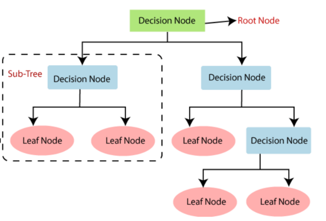
Figure 1. The process of the decision tree

3. Methodology (Implementation)

We use the machine learning algorithm to deal with credit risk. Specifically, we use the following machine learning methods: SVM, KNN and DTs. Before introducing the specific application of the algorithm, we first formalize the question.

\( T=\lbrace ({x_{1}}, {y_{1}}),({x_{2}}, {y_{2}}),…, ({x_{N}}, {y_{N}}), \rbrace \)

Denote T as training data, where \( {x_{i}} ∈X ⊆ {R^{n}} \) is the eigenvector of the specimen; \( {y_{i}}∈ y=\lbrace 0, 1\rbrace \) is the category of the instance, where 0 is not default and 1 is the default; \( i=1, 2,…, N \) ; eigenvector of the instance \( x \) . The aim is to successful classify whether people would default or not. More specifically, A classifier would be built for \( f(x) \) , and classifier’s output would either be 0 or 1.

3.1. SVM

The algorithm would be the following.

First, choose penalty parameter [11] \( ∁ \gt 0 \) , conducting and convex quadratic programming problem.

\( \begin{matrix}min \\ a \\ \end{matrix} \frac{1}{2}\sum _{i=1}^{n}\sum _{i=1}^{n}aiajyiyj(xi × xj)- \sum _{i=1}^{n}aj t. ∑\_(i=1)\text{^}n▒〖aiji =0〗 \)

\( 0 ≤ai ≤C, i=1, 2, … , N \)

Second, find the best solution \( {a^{*}}={(a_{1}^{*}, a_{2}^{*}, …, a_{N}^{*})^{T}} \)

Third, pay a circle \( ξi, \) which makes the aimed function change from \( \frac{1}{2}{‖w‖^{2}} \) to

\( \frac{1}{2}{‖w‖^{2}}+ C\sum _{i=1}^{N}ξi \)

\( st. yi(w×xi +b)≥1-ξi, i= 1, 2, …, N \)

\( ξi ≥0, i= 1, 2, …, N \)

Due to it being a convex quadratic programming problem, the solution of ( \( w, b, ξ) \) exists. It can be proved that the key for w is unique, but for b is not; it would be in a range.

3.2. KNN

First, based on the given distance measure, find K nearest points in the training data T, the neighborhood of x covering the k points is calculated N_k (x)_;

Second, based on the Classification decision rule(such as majority voting ), deciding the class y for x in N_k (x)

\( y=arg{ \frac{max}{cj} \sum _{xi ∈ Nk (x)}I (yi=cj), i=1, 2, …, N; j=1, 2,…, K } \)

In the following equation, I is the indicator function, which means when \( yi=cj \) , I either be 1 or 0.

The KNN is a unique situation that k = 1, called the KNN algorithm. For the input instance point (eigenvector) x, the nearest neighbours method treats the class of the closest point to x in the training data set as the x class.

3.3. Generate a CART Decision Tree

Based on the training datasets, start from the root rode, did the following recursively for each node, which conducts the decision tree. First, let each node dataset be D and calculate the Gini index [12] for the existing feature. In these moments, based on every feature A and every possible value A, based on the sample point A = A. Dividing the D into two parts, D1 and D2, based on the ‘right’ or ‘wrong’, and calculating the Gini index when A = A. Second, Choosing the lowest Gini index and its corresponding segment point to be the best feature and segment point across all the possible feature A with all the possible segment points. Based on those best feature points, generate two child nodes from the current node and allocate those train datasets based on the feature points. Third, invoking (1) and (2) from two child nodes until it satisfies the condition precedent. Finally, generate a CART decision tree.

The algorithm stops calculating when the number of samples in the node is less than the predetermined threshold, the Gini index of the sample set is less than the predetermined threshold (the pieces belong to the same class), or there are no more features.

Firstly, the Gini index of each feature is calculated, and the optimal quality and its optimal segmentation point are selected. The symbols of Example 5.2 are still adopted. Al, A2, A3 and A4, respectively represent the four characteristics of age, having a job, owning a house and credit situation, and the values of 1, 2 and 3 illustrate youth, middle age and old age.1,2 means yes and no for having a job and owning your own home, and 1,2,3 means very pleasing, pleasing and average for credit.

The following equation is the definition of the probability distribution for the Gini index. Assume they have K classes, and the sample points belong to the K’s class named \( {p_{k}} \) .

\( Gini(p)= \sum _{k=1}^{K}{p_{k}}(1- {p_{k}})=1- \sum _{k=1}^{K}P_{k}^{2} \)

Based on the given sample set named D, the equation would be the following:

\( Gini(D)= {\sum _{k=1}^{K}(\frac{|{C_{k}}|}{|D|})^{2}} \)

3.4. Data Set

This section will explore and address the approach of preparing the dataset from Kaggle [13]. A description of the data structure is presented first. To deal with high-dimension data, they would be using different aspects to analyze the data throughout the selected data.

3.5. Dat

Data is obtained from Kaggle, which contains 35282 observations with twelve variables. There is a combination of categorical variables and numerical variables, where four variables are categorical and eight are numeric. Some of the data contains missing values. To solve this problem, Simple Imputer has been used in Python. The standard five nearest neighbors are applied, because of the combinations of the categorical and numerical database.

4. Preprocessing

The following 4 sub-topics shows how we are processing the data that we have got to the models.

4.1. Meaning of the Variable

Table 1. The meaning of the variables

The Table 1 shows the meaning of each variable, making easier to understand each variable’s meaning.

4.2. Missing Value

In this dataset, some of the values are missing in the data, to complete the table, we have used the Simple Imputers inside the Scikit learn to find the total amount of the missing value and use the strategy of the mean to fill the missing value, so the total amount of the missing value changed from Table 2 to Table 3.

Table 2. The sum of the missing value in different categories (Before)

Table 3. The sum of the missing value in different categories (After)

4.3. Train-test Split

The computer does not know how to calculate with the data that you have given to them. In this case, we need to provide two categories of datasets, one of the datasets is called a train dataset, which simply means that this type of dataset is used to assist the computer in learning. To know the dataset people, want. It is similar to students that need to do a lot of questions to know how to get a high grade in the exam. The other dataset is called the test dataset, which after the computer completes the train dataset, can provide the final result of the experiment. This is similar to the students that do the topic assessment, and the teacher are marked and gives a grade to the students. In machine learning (ML), we have split the whole dataset into two types: 70% of the entire datasets are train datasets and the remaining 30% are test datasets.

4.4. Identifying the Categorical Variables

The computer could not identify and calculate the categorical variables without exchanging the dataset for numeric variables. To exchange the variables, it needs to use the replace function to trade the character string to a number. In this case, it would change the categorical variables to numeric variables.

5. Result

In this paper, three methods, Support Vector Machine (SVM), K-Nearest Neighbors (KNN) and Decision Tree model (DTs) have been compared with the effectiveness and accuracy of the result. MAE, MSE and AUC would be the primary standards and measurements for their classification performance.

5.1. MAE

The mean absolute error (MAE) is defined the average variance between the significant values in the dataset and the projected values in the same dataset. [14] The results for the MAE in the methods of SVM, KNN and DTs used in machine learning are shown in the Table 4 and Tables 5.

5.2. MSE

Mean-square error (MSE) linear estimation is a topic of fundamental importance for parameter estimation in statistical learning.[15] The results for the MSE in the methods of SVM, KNN and DTs used in machine learning are shown in Table 4 and Table 5. The results for the AUC in the methods of SVM, KNN and DTs used in machine learning are shown in the Table 4 and Tables 5.

5.3. AUC

The receiver operating characteristic curve (ROC)[16] is a graph showing the performance of a classification model at all classification thresholds. Area under the ROC Curve (AUC) measures the entire two-dimensional area underneath the ROC as a whole curve (think integral calculus) from (0,0) to (1,1).

Table 4. The classification performance

Table 4 shows the comparison of three methods (KNN, DTs and SVM) by using 3 standard measurements to monitor their performance on classification.

5.4. Evaluation of the Dataset

According to the result that have been shown in table 4, the best method for this dataset would be the Decision Trees (DTs), since for both the MAE and MSE, it got the lowest number compared to 2 other methods for MAE and MSE, the lower the number, the higher the accuracy. For the AUC, which is exactly the opposite, the higher the number, the higher the accuracy. The DTs method got 0.917, which is highest across the three ways.

5.5. SVM

As during the result of the SVM, several parameters are needed to debug and find the best result. The parameters of the SVM include the kernel, gamma, shrinking and penalty parameter(C). Inside the kernel; it contains ‘linear’, ‘poly’, ‘Rbf’, ‘sigmoid’, and ‘precomputed’ where only ‘linear’, ‘poly’, ‘Rbf’, and ‘sigmoid ‘can be used in this paper.

Table 5. Result when C equals to 1

Table 5 shows that the penalty parameter(C) equals to 1, which would be the number for the Kernel.

Table 6. Result when C equals to 8

The table 6 shows that the penalty parameter(C) equals to 8, which would be the number for the Kernel.

Based on the 2 sets of tables, the conclusion that can be made would be the Rbf would be the best kernel as it shows the best results between both tables for the penalty parameter(C). It shows generally higher results across four different categories. In this case, we can conclude that the best outcome would be Rbf with the penalty parameter(C) equals to 8.

6. Conclusion

The paper explores credit risk prediction using machine learning models, specifically Support Vector Machine (SVM), K-Nearest Neighbors (KNN), and Decision Tree (DT) models. After implementation and comparison, Decision Trees demonstrated the highest accuracy in predicting credit risk. The dataset, obtained from Kaggle, underwent preprocessing steps, including handling missing values and transforming categorical variables. Evaluation metrics such as MAE, MSE, and AUC were employed, with Decision Trees proving to be the most effective method for the given dataset. Additionally, the study delves into parameter tuning for SVM, highlighting the Rbf kernel with a penalty parameter (C) of 8 as the optimal configuration. In conclusion, Decision Trees, among the evaluated methods, emerge as the preferred choice for credit risk prediction in this study.

References

[1]. Crouhy, M., Galai, D., & Mark, R. (2000). A comparative analysis of current credit risk models. Journal of Banking & Finance, 24(1-2), 59-117.
[2]. Duignan, B. (2023, 8 14). financial crisis of 2007–08. Retrieved from Encyclopedia Britannica: https://www.britannica.com/money/topic/financial-crisis-of-2007-2008#ref342321
[3]. Mathur, A., & Foody, G. M. (2008). Multiclass and binary SVM classification: Implications for training and classification users. IEEE Geoscience and remote sensing letters, 5(2), 241-245.
[4]. Ding, S., Hua, X., & Yu, J. (2014). An overview on nonparallel hyperplane support vector machine algorithms. Neural computing and applications, 25, 975-982.
[5]. Sifaou, H., Kammoun, A., & Alouini, M. S. (2019, December). Phase transition in the hard-margin support vector machines. In 2019 IEEE 8th International Workshop on Computational Advances in Multi-Sensor Adaptive Processing (CAMSAP) (pp. 415-419). IEEE.
[6]. Cortes, C., & Vapnik, V. (1995). Support-vector networks. Machine learning, 20, 273-297
[7]. Zhang, Z. (2016). Introduction to machine learning: k-nearest neighbors. Annals of translational medicine, 4(11).
[8]. Mahesh, B. (2020). Machine learning algorithms-a review. International Journal of Science and Research (IJSR). [Internet], 9(1), 381-386.
[9]. Quinlan, J. R. (1986). Induction of decision trees. Machine learning, 1, 81-106.
[10]. Viraj_Lakshitha. (2021, 1 21). What is a Decision Tree in ML? Retrieved from medium.com: https://vitiya99.medium.com/what-is-a-decision-tree-in-ml-5bd76efc2232
[11]. Imam, T., Ting, K. M., & Kamruzzaman, J. (2006). z-SVM: An SVM for improved classification of imbalanced data. In AI 2006: Advances in Artificial Intelligence: 19th Australian Joint Conference on Artificial Intelligence, Hobart, Australia, December 4-8, 2006. Proceedings 19 (pp. 264-273). Springer Berlin Heidelberg.
[12]. Tangirala, S. (2020). Evaluating the impact of GINI index and information gain on classification using decision tree classifier algorithm. International Journal of Advanced Computer Science and Applications, 11(2), 612-619
[13]. TSE, L. (2020). Credit datasets. Retrieved from Kaggle: https://www.kaggle.com/datasets/laotse/credit-risk-dataset
[14]. Manoj, S. O. (2022). 17 - FWS-DL: forecasting wind speed based on deep learning algorithms. In S. O. Manoj, Artificial Intelligence for Renewable Energy Systems (pp. 353- 374). Woodhead Publishing.
[15]. Theodoridis, S. (2020). Machine Learning A Bayesian and Optimization Perspective. Academic Press.
[16]. Team, g. d. (2022, 7 18). Classification: ROC Curve and AUC. Retrieved from developers. google: https://developers.google.com/machine-learning/crash-course/classification/roc-and-auc.
Cite this article
Wu,C. (2024). Credit risk unveiled: Decision trees triumph in comparative machine learning study. Applied and Computational Engineering,79,174-181.
Data availability
The datasets used and/or analyzed during the current study will be available from the authors upon reasonable request.
Disclaimer/Publisher's Note
The statements, opinions and data contained in all publications are solely those of the individual author(s) and contributor(s) and not of EWA Publishing and/or the editor(s). EWA Publishing and/or the editor(s) disclaim responsibility for any injury to people or property resulting from any ideas, methods, instructions or products referred to in the content.
About volume
Volume title: Proceedings of the 4th International Conference on Signal Processing and Machine Learning
© 2024 by the author(s). Licensee EWA Publishing, Oxford, UK. This article is an open access article distributed under the terms and
conditions of the Creative Commons Attribution (CC BY) license. Authors who
publish this series agree to the following terms:
1. Authors retain copyright and grant the series right of first publication with the work simultaneously licensed under a Creative Commons
Attribution License that allows others to share the work with an acknowledgment of the work's authorship and initial publication in this
series.
2. Authors are able to enter into separate, additional contractual arrangements for the non-exclusive distribution of the series's published
version of the work (e.g., post it to an institutional repository or publish it in a book), with an acknowledgment of its initial
publication in this series.
3. Authors are permitted and encouraged to post their work online (e.g., in institutional repositories or on their website) prior to and
during the submission process, as it can lead to productive exchanges, as well as earlier and greater citation of published work (See
Open access policy for details).