1. Introduction

A key factor for training a successful machine learning model has always been the existence or gathering of comprehensive datasets covering all the features one wish elicit conclusions from. Sometimes, it is a matter of time and effort for one to collect such datasets, but there are also cases where these data are scattered across multiple locations guarded behind laws aimed to protect privacy. For example, patient records are strictly protected by law, consequentially hospitals only have access to a portion of the total population when training machine learning models for tasks such as medical imaging diagnosis. This limitation can be realized from the relatively small size of accessible dataset, as well as its lack of capability to represent the true distribution. Ideally, collaboration between hospitals would result in a much higher quality model, but this is prohibited by the protected nature of these medical data.

Federated Learning (FL) [1] offers an effective approach for training decentralized machine learning models, enabling cross-silo/cross-device collaboration while preserving data privacy. In this setting, a global model is trained on a central server by aggregating training results of local clients. This paradigm requires no communication in the data layer, but instead processes all the model parameters trained on local data in some way to produce a comprehensive global model capturing the local distributions. However, challenges regarding data imbalance comes naturally. Data heterogeneity, or non-independent and identically distributed (non-IID) data poses challenges to the performance of FL models, potentially skewing model performance significantly. Data imbalances can significantly hinder the performance of machine learning models by reducing their accuracy and reliability when applied to diverse real-world scenarios. This reduction in model generalization can lead to suboptimal decisions and inefficiencies in various applications. Biased models can severely undermine trust in critical systems such as healthcare. If left unchecked, these models may produce life-altering outcomes, particularly affecting underrepresented groups.

There have been algorithms designed to combat the negative consequences of non-IID data, as well as studies on the efficacy of these algorithms for different machine learning tasks and levels of non-IID-ness. However, to the extent of our knowledge, there hasn’t been a structured, experimental study on the performances of FL algorithms under extreme non-IID conditions across different model types. The concept of extreme will be defined in detail in a following section of the paper. Not only were three state-of-the-art FL algorithms chosen to be the target of this study, namely FedAvg [1], FedProx [2], and SCAFFOLD [3], three model types have been selected for further comparisons and investigations, including ResNet [4], AlexNet [5], and DenseNet [6].

The performance of these models and algorithms will be compared in various scenarios characterized by different degrees of data imbalance as well as different numbers of local training steps - a hyperparameter lacking comprehensive experiments to prove its importance and impact on model training. By analyzing the outputs of the experiments, including model accuracies and training time, this paper aims to systematically study the relationship between FL algorithms, neural networks, and their respective datasets.

The findings of this paper provide valuable insights into the behavior of these models and optimization algorithms in the presence of data imbalances and under different training scenarios, guiding the selection of appropriate techniques for FL. Through the different combinations of hyperparameters, this paper aims to establish a thorough understanding of the behaviors of current FL algorithms, contributing to the future development of more efficient and reliable algorithms capable of handling non-IID data distributions encountered in training settings.

2. Related Works

There have been extensive studies regarding the impact of heterogenous data in the context of distributed learning. Regarding class imbalance, Xiao et al. [7] formulated a systematic approach to its definition, specifically categorizing class imbalance in FL into four scenarios based on two proposed metrics: Global Imbalance Degree using Multiclass Imbalance Degree (MID) and Local and Global Relation using Weighted Cosine Similarity (WCS). Results showed that a higher MID led to worse global model performance, and a lower WCS not only degraded performance but also slowed down model convergence by introducing optimization fluctuations. Xiao et al.’s work highlights the distinctions between and impacts of global and local imbalances, suggesting that solutions targeting heterogeneity need to tackle both appropriately to improve FL performance.

One of the solutions to address the class imbalance problem came from Wang et al. [8], which includes two key components: inferring the degree of global class imbalance from gradient magnitudes and sample quantities of different classes, and a loss function called Ratio Loss where it introduces class-specific weights based on gradient ratios of classes to modify the cross-entropy loss. Ratio Loss increases the contribution of minority classes to the overall loss to mitigate class imbalance without the need for clients to share local data distributions.

Li et al. [9] presented a comprehensive study on four different FL algorithms under non-IID settings, filling in the hole for a systematic evaluation and comparison of the algorithms, some of which proposed to address the challenges of working with non-IID data. This paper categorizes data heterogeneity into three types: label distribution skew, feature distribution skew, and quantity skew. Experiments regarding each of the three types were conducted using multiple image datasets, providing insights to the strengths and weaknesses of the targeted algorithms. The systematic classification of heterogeneity sheds light on the nuances that can exist within non-IID datasets that should be paid attention to when choosing a FL algorithm.

Extending beyond boundaries of the studies by Li et al., this paper aims to further investigate the impact of various hyperparameters and model architectures on the performance of FL algorithms in non-IID scenarios. This paper seeks to provide an even more comprehensive understanding of the factors that play into the success or failure of FL algorithms in non-IID settings, with the aim of helping researchers make better informed decisions when selecting FL algorithms to use but also presenting insights for the development of more robust algorithms.

3. Federate Learning Algorithms

Here are the summaries of the FL algorithms relevant to the paper including FedAvg, FedProx, and SCAFFOLD. The latter two are variations of the first with changes made aimed to mitigate accuracy loss caused by data imbalances. With FedAvg as the baseline, this paper studies its comprehensive performance when using different combinations of hyperparameters, as well as compares how its variations - FedProx and SCAFFOLD - do against their predecessor. FedProx and SCAFFOLD differ from FedAvg by changing the loss function or adding additional parameters to restrict the updates of the model. There exists other algorithms and techniques that accomplish similar goals of dealing with non-IID data such as partial/full model personalization, which is out of the scope of this paper.

3.1. FedAvg

Federated Averaging (FedAvg) is one of the most popular algorithms used in FL. The framework is shown in Figure 1. The algorithm starts by having the central server send a global model to all the clients participating in this round of training. After all training is finished locally, these models are sent back to the server for aggregation which for FedAvg is a straightforward average of all models. The algorithm allows the global model to be influenced by all local data distributions otherwise not accessible amongst all clients. Although an effective solution to data accessibility problems, FedAvg is susceptible to non-IID data as the average operation cannot eliminate the negative effects of data imbalances. If there are certain classes that are excessively represented across clients, then FedAvg can become biased and show worse performance on under-represented classes.

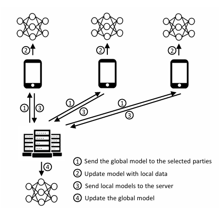
Figure 1. The FedAvg architecture [1].

3.2. FedProx

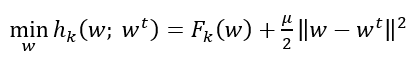
FedProx attempts to tackle the challenges brought about by heterogeneous data distributions by extending upon FedAvg. FedProx adds an additional L2 regularization term to the local objective function, restricting the local models to stray too far from the global model transmitted at the beginning of every communication round. This proximal term - hence the name FedProx - limits the size of local updates by limiting the distance between the local and the global model, enabling FedProx to be more stable and converge faster compared to FedAvg, especially in the non-IID settings.

(1)

Equation (1) shows the modified local objective function for FedProx. \( {F_{k}} \) represents the original local objective function for client k; \( w \) represents local model parameters; \( {w^{t}} \) represents global model parameters at communication round t; \( μ \) is the proximal term coefficient. The proximal term also allows clients to perform more varying numbers of local updates with less worry about its effect on later aggregations. A hyperparameter μ is introduced to control the extent of the L2 regularization, typically chosen to be in the range between 0.001 to 0.1. For this paper, this value is set to 0.01 and never changes.

3.3. SCAFFOLD

SCAFFOLD (Stochastic Controlled Averaging for Federated Learning) is another algorithm designed to combat data imbalances in FL (Figure 2). The key idea behind SCAFFOLD is the introduction of control variates, additional parameters used to correct client-drift during local updates. Like how the model is trained in FL, the control variates are trained in a similar fashion. The server keeps a global control variate that gets transmitted to each client every communication round. During local training, the client updates its copy of the global control variate and updates the weights of the model while considering the difference between the locally updated and global control variates. This reduces the effect of client drift by aligning the local updates more with the global objective. At the end of the local training, the local control variates are sent back to the server for aggregation.

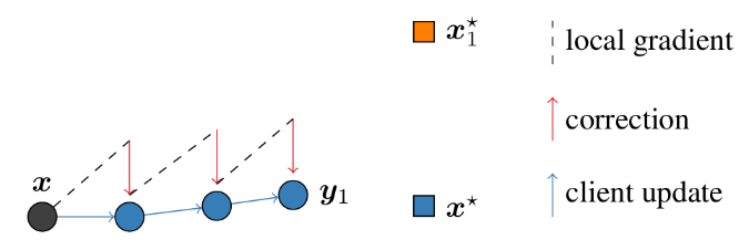
Figure 2. Correction term of SCAFFOLD to prevent client drift. \( {{x_{1}}^{*}} \) represents local optimum, \( {x^{*}} \) represents true optimum [3]

4. Models

The models chosen for this study are ResNet50, AlexNet, and DenseNet. The choices were made with the aim of covering a wide range of neural networks suitable for the dataset CIFAR-10, an image classification dataset consisting of 60,000 32x32 color images in 10 classes.

ResNet50: ResNet [4], or residual network, introduces the concept of skip connections as a solution to the vanishing gradient problem that occurs in deep neural networks. As the model goes through back propagation to update its weights, gradients can become extremely small due to the nature of their calculations, preventing weights in earlier layers from being updated significantly. Skip connections allow for a much deeper network to be trained. Specifically, ResNet50 contains 50 layers, a total of about 23.7 million parameters.

AlexNet: AlexNet [5] represents a relatively basic deep convolutional neural network. Through the introduction of ReLU and dropout for regularization, AlexNet was significant in its contribution to deep learning for computer vision. This paper’s implementation added batch normalization, originally introduced after the creation of AlexNet, as well as some adjustments to fit the smaller image size of CIFAR-10. The paper’s implementation of AlexNet has around 7 million parameters.

DenseNet121: With dense connectivity between layers in a feed-forward fashion, DenseNet [6] allows feature reuse throughout the network, thus creating a more compact model. DenseNet121 is a smaller implementation of DenseNet, with around 7.8 million parameters taking into account the changes made to fit CIFAR-10.

5. Experimental Setup

5.1. Dataset

All experiments are performed on the CIFAR-10 dataset [10], consisting of 60,000 color images of 10 classes, with the task being image classification. To extend upon the existing data, this paper uses torchvision.transforms for data augmentation, specifically utilizing RandomCrop and RandomHorizontalFlip, adding variations of the original images.

5.2. Hyperparameter setup & evaluation metrics

For all experiments, the batch size was set to 128, and the learning rate was set to 0.001. The number of communication rounds is 40 for both ResNet50 and AlexNet, and 25 for DenseNet121 due to its increased time costs. The number of clients participating in FL is not a hyperparameter focused by this paper and is set to 5. Cross entropy loss is used as the loss function, and Adam as the optimizer. Specifically, for FedProx, the proximal hyperparameter μ is set to 0.01. Hyperparameter-wise, the main targets of this study are number of local steps [1, 3, 5] and alpha [0, 0.05, 0.1] which controls the extent of imbalance generated by Dirichlet distribution. The definition of alpha = 0 will be established in a later section as it is originally undefined.

The performances of the models will be evaluated by two metrics, the first being their accuracies on the test set (10,000 out of 60,000 images), and the second being time taken to finish training. As one of the goals of this paper is to help make more informed decisions when choosing which algorithms to use, training cost in the form of time spent is included as a metric. Accuracy is calculated based on the correct labels predicted out of the total number of test images. Time is measured from before the server sets up anything until model evaluation on the test set finishes after the last round of communication.

5.3. Data partitioning and simulating data imbalances

Following the most common and reliable method of simulating data imbalances, the CIFAR-10 dataset is partitioned among the clients using Dirichlet distributions for all experiments conducted in this study. The Dirichlet distribution allows control of the level of imbalance across clients by adjusting the parameter alpha. The lower the value of alpha, the more skewed the distribution is, therefore simulating different levels of non-IID scenarios. Figure 3 shows examples of such distributions. As mentioned in a previous section, alpha = 0 is not strictly defined when it comes to Dirichlet distributions. To simulate the most extreme form of imbalance, this paper defines alpha = 0 to be the behavior of the distribution as alpha gets infinitely close to 0, i.e. all images of the same class belong to the same client. Since the number of classes and the number of clients is constant throughout the experiments, the implementation of the alpha = 0 behavior simplifies randomly assigning images of 2 classes to each of the 5 clients, a total of 10 classes.

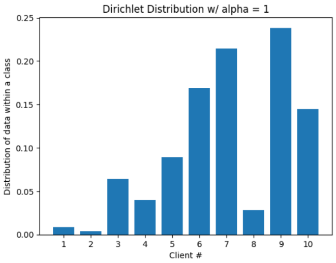
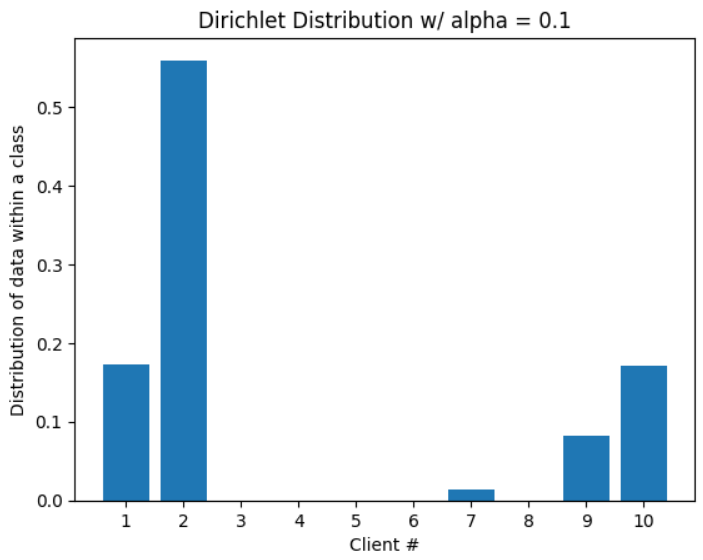
Figure 3. Dirichlet distributions parameterized by alpha (Picture credit : Original)

6. Results Analysis

Table 1 contains all aggregated experimental results, with all numbers rounded to one decimal place. Each experimental configuration was performed five times, where the results were averaged, and standard deviations calculated for accuracies. All experiments were run on the University of Virginia CS server, which has 8 NVIDIA RTX A6000 GPUs.

6.1. Impact of non-IID data distributions

The Dirichlet distribution parameter α has a significant influence on the performances of models across all different combinations of FL algorithms and other hyperparameters. A trend of improved accuracy can be observed as α increases from 0 (custom defined as extreme non-IID) to 0.1 (relatively balanced). When α = 0, results show that the accuracies are generally low across all configurations, ranging from 22.3% using ResNet50 and FedAvg with local step = 1, to 54.7% using AlexNet and FedProx with local step = 1. We can see that data imbalance is in fact detrimental to model training results and is certainly something that needs to be addressed. Increasing α from 0 to 0.05 usually yields substantial accuracy increases. For example, when using ResNet and FedAvg, the accuracy for local steps = 5 increased from 36.9% to 54.4%. There’s only a modest increase in data balance from α = 0 to 0.05, but what this demonstrates is that such a minor increase can lead to significant performance gains (Table 1).

It is expected that data partitions of α = 0.1 yield the highest accuracies, and the results prove to be consistent with such expectation. The highest accuracy for ResNet was achieved by SCAFFOLD with local steps = 3, highest for AlexNet and DenseNet achieved by FedAvg with local steps 5, all with α = 0.1. These results demonstrate the importance of having balanced distributions in data used for model training.

Table 1. Test accuracies and time costs of all configurations. Five trials were run for all experiments, reporting the average and standard deviation all rounded to one decimal place. Bolded cells represent highest accuracy within the same configuration (row)

6.2. Effect of local training steps

Results show that behaviors exhibited by the target models and FL algorithms vary under the change of local training steps. The differences reveal interactions between the FL algorithms and the hyperparameter in question, bringing attention to the importance of choosing the right value befitting of the corresponding algorithm.

For both FedAvg and SCAFFOLD, the relationship between number of local training steps and model accuracy generally resembles a positive correlation. There are occasions when results with local steps = 3 beat results with local steps = 5, but not once does local step = 1 achieve the highest accuracy. Having a higher number of local training steps means clients are likely to be closer to their local optima, capturing more client-specific features. FedAvg does a good job of smoothing out individual client biases during the averaging process; SCAFFOLD uses control variates to correct for client drift, allowing it to handle more iterations of local training effectively. There is little evidence to show that the amount of increase in accuracy when increasing the number of local steps has anything to do with the imbalance degree. Increases of less than 10% and more than 20% can be seen scattered in the results with no apparent trend. With respect to FedAvg and SCAFFOLD, one can safely conclude that allowing more local training before aggregation is beneficial to model accuracies, though varying at different amounts.

On the other hand, it is interesting to note that FedProx rarely benefits from an increase in local training steps, even showing almost consistently worse performance as the number increases. Taking the results from using ResNet, the model accuracy always decreases as local steps increases with no exception. Intuitively, this could be explained by the nature of the algorithm, where the proximal term goes against the practice of having multiple local training steps. The L2 regularization acts more as a restriction over multiple local steps, hindering the model from capturing the client-specific patterns, ultimately disabling the global model to effectively aggregate the information learned.

6.3. Algorithm comparison

From the number of configurations that a FL algorithm had achieved the highest testing accuracy for, FedAvg and SCAFFOLD do equally as well, while FedProx struggles to match the other two. FedAvg demonstrates solid performance across the different configurations, struggling mostly with lower α values and local steps. Despite FedAvg not addressing the problem of data imbalance in its algorithm, results show that it does not fall significantly behind the other two, sometimes even beating them in cases of lower α values. SCAFFOLD performs extremely well for ResNet, topping the chart for six out of nine configurations. A potential for such a behavior could be that SCAFFOLD’s approach to correct client drift is beneficial to deep neural networks, and possibly working synergistically with skip connections, thus improving information flow during the learning process and yielding more effective training even in non-IID scenarios. Results of FedProx contain a very interesting trend, that although it generally doesn’t perform as good as FedAvg and SCAFFOLD, it exceeds in the extreme non-IID scenario (α = 0) when local step = 1. For all three models, FedProx performs the best, even reaching an accuracy of 54.7% when the others are only around 24%. This suggests that FedProx is most suitable for minimum local training and highly skewed data distributions.

6.4. Model comparison

Amongst the three studied models, ResNet showed the most improvements with the increase of α, AlexNet proved to be the most robust to data imbalances with the highest accuracies for α = 0, and DenseNet sitting somewhere between the former two. These results show that complex model architectures, such as ResNet compared to AlexNet, might be more prone to data imbalances.

6.5. Computational costs

The second metric of this paper is the time cost of training using each configuration, aimed to provide insights towards the question of how much more resources are being consumed for an increase in accuracy, if at all, in non-IID scenarios. FL algorithm wise, FedProx generally takes the longest time due to the calculations of the proximal term. Between FedAvg and SCAFFOLD, the numbers are rather similar, with SCAFFOLD usually taking a bit longer as it requires some extra calculations with the control variates. Model wise, AlexNet is the fastest to train due to its simpler architecture, and DenseNet being the slowest because of its dense connectivity and memory costs. This comparison is based on normalized time costs by dividing the average time taken per communication round by the number of parameters in millions, presented in Table 2.

Table 2. Metadata of experimental results

7. Conclusion

This comprehensive study of FL algorithms under various non-IID settings, specifically the analysis of test accuracies and time costs of models with different combinations of data imbalance levels, number of local training steps, and model types, presented several insights. First, the degree of imbalance characterized by the parameter significantly impacts model performances across all configurations, consistently causing an increase in accuracy as α itself increases. Second, the number of local training steps demonstrated its different effects depending on the FL algorithm used, benefiting FedAvg and SCAFFOLD but mostly detrimental towards models utilizing FedProx. Third, model architecture plays an important role in handling data imbalances. Simpler models are more robust towards skewed data distributions and complex models prove to suffer more from them. Further research questions come naturally from this study, such as adding more varying hyperparameters in the configuration and studying the differences in behaviors. The number of clients was restricted to five throughout this study but could be changed to see how it impacts performance. Findings of this paper contribute to a deeper understanding of FL algorithms’ performances under various non-IID conditions and offer insights for practitioners in selecting fitting configurations for specific use cases.

References

[1]. McMahan, B., Moore, E., Ramage, D., Hampson, S., & y Arcas, B. A. (2017, April). Communication-efficient learning of deep networks from decentralized data. In Artificial intelligence and statistics (pp. 1273-1282). PMLR.
[2]. Li, T., Sahu, A. K., Zaheer, M., Sanjabi, M., Talwalkar, A., & Smith, V. 2020. Federated optimization in heterogeneous networks. Proceedings of Machine learning and systems, 2, 429-450.
[3]. Karimireddy, S. P., Kale, S., Mohri, M., Reddi, S., Stich, S., & Suresh, A. T. 2020, November). Scaffold: Stochastic controlled averaging for federated learning. In International conference on machine learning (pp. 5132-5143). PMLR.
[4]. He, K., Zhang, X., Ren, S., & Sun, J. 2016. Deep residual learning for image recognition. In Proceedings of the IEEE conference on computer vision and pattern recognition (pp. 770-778).
[5]. Krizhevsky, A., Sutskever, I., & Hinton, G. E. 2012. Imagenet classification with deep convolutional neural networks. Advances in neural information processing systems, 25.
[6]. Huang, G., Liu, Z., Van Der Maaten, L., & Weinberger, K. Q. 2017. Densely connected convolutional networks. In Proceedings of the IEEE conference on computer vision and pattern recognition (pp. 4700-4708).
[7]. Xiao, C., & Wang, S. (2021, December). An experimental study of class imbalance in federated learning. In 2021 IEEE Symposium Series on Computational Intelligence (SSCI) pp. 1-7.
[8]. Wang, L., Xu, S., Wang, X., & Zhu, Q. 2021. Addressing class imbalance in federated learning. In Proceedings of the AAAI Conference on Artificial Intelligence Vol. 35, No. 11, pp. 10165-10173.
[9]. Li, Q., Diao, Y., Chen, Q., & He, B. 2022. Federated learning on non-iid data silos: An experimental study. In 2022 IEEE 38th international conference on data engineering (ICDE) pp. 965-978.
[10]. Krizhevsky, A., & Hinton, G. 2009. Learning multiple layers of features from tiny images.Handbook of Systemic Autoimmune Diseases, 1(4).
Cite this article
Zheng,W. (2024). Comparative analysis of federated learning algorithms under extreme non-IID conditions for computer vision. Applied and Computational Engineering,86,168-176.
Data availability
The datasets used and/or analyzed during the current study will be available from the authors upon reasonable request.
Disclaimer/Publisher's Note
The statements, opinions and data contained in all publications are solely those of the individual author(s) and contributor(s) and not of EWA Publishing and/or the editor(s). EWA Publishing and/or the editor(s) disclaim responsibility for any injury to people or property resulting from any ideas, methods, instructions or products referred to in the content.
About volume
Volume title: Proceedings of the 6th International Conference on Computing and Data Science
© 2024 by the author(s). Licensee EWA Publishing, Oxford, UK. This article is an open access article distributed under the terms and
conditions of the Creative Commons Attribution (CC BY) license. Authors who
publish this series agree to the following terms:
1. Authors retain copyright and grant the series right of first publication with the work simultaneously licensed under a Creative Commons
Attribution License that allows others to share the work with an acknowledgment of the work's authorship and initial publication in this
series.
2. Authors are able to enter into separate, additional contractual arrangements for the non-exclusive distribution of the series's published
version of the work (e.g., post it to an institutional repository or publish it in a book), with an acknowledgment of its initial
publication in this series.
3. Authors are permitted and encouraged to post their work online (e.g., in institutional repositories or on their website) prior to and
during the submission process, as it can lead to productive exchanges, as well as earlier and greater citation of published work (See
Open access policy for details).