1. Introduction

Panoramic image stitching is an important research direction in the field of computer vision, he can stitch multiple images into a panoramic image, which is particularly important for commercial and artistic value, such as virtual reality, augmented reality and satellite image processing and many other applications. With the advent of digital cameras, the desire to create full panoramic images has become stronger, and the importance of automatic image stitching has come to the fore [1]. However, in the process of image stitching, the inaccuracy of feature point matching and the existence of external points often lead to the failure of the stitching result. Therefore, it is an important purpose of this study to find the most suitable method to effectively exclude the outer points.

In today's increasingly tight computing resources, maintaining high efficiency and high precision is a challenge for image Mosaic technology. Therefore, it is of great research significance and value to find out the algorithm with the best performance, which not only provides theoretical value for subsequent academic research, but also optimizes today's stitching technology. Common methods for model estimation include random sampling consistency algorithm (RANSAC), least square method and least median square method (LMedS). RANSAC is very robust and removes outliers by randomly selecting sample points and iteratively optimizing the model. In contrast, the least squares method estimates model parameters by minimizing the sum of squares of residuals, but is highly sensitive to external points [2]. LMedS attempts to reduce the influence of the maximum outlier on the model estimation through the median statistic and enhance the robustness of the model.

Although the advantages and disadvantages of these model estimation methods have been explored, there is still a research gap in the performance discussion of these algorithms in practical applications. Therefore, this paper will compare the performance of different methods such as RANSAC, least square and LMedS in panoramic image Mosaic, and explore their efficiency in handling outliers and the quality of Mosaic results. Finally, the most suitable model estimation method is given by comparing the data of different algorithms.

2. Related work

In order to improve the accuracy and efficiency of image Mosaic, many scholars have proposed various feature matching and model estimation methods. At present, the main methods are feature point matching, model estimation and deep learning.

2.1. Feature point matching

SIFT (Scale invariant Feature Transform) and SURF (Accelerated Robust feature) are two algorithms that detect local feature points to achieve feature matching. Lowe's study showed that SIFT is invariant to rotation and scale changes, which significantly improves the stitching quality, but it is not sufficiently robust and unique in feature matching [3]. In addition, SURF algorithm proposed by Bay et al. provides a faster feature computation speed than SIFT, which relies on image Gaussian scale space analysis [4]. ORB is a more computationally efficient alternative that is widely used in real-time image stitching. It combines FAST keypoint detection with BRIEF descriptors to make the feature matching process more efficient. However, in complex scenarios, the matching accuracy may decrease.

2.2. Model estimation

Since its introduction, RANSAC has become a standard method for outlier detection and model estimation. Torr and Zisserman demonstrated that RANSAC can also effectively estimate the homologous matrix when dealing with scenes with high ratio exceptions, thereby improving the stitching effect [5]. In order to improve robustness to outliers, In addition, the least square method, as a classical estimation method, has been widely used because of its simple mathematics and high computational efficiency. However, when there are a large number of external points, the performance of least squares degrades, resulting in unreliable model estimates. To solve this problem, the researchers introduced more powerful methods, such as LMedS (minimum median squared), designed to improve the model's resistance to outliers. In order to improve the robustness of the outlier, LMedS selects the median as the estimator to reduce the influence of the maximum outlier on the model.

2.3. Deep learning method

With the rapid development of deep learning, researchers begin to explore its application in panoramic image Mosaic. For example, convolutional neural networks (CNNS) have been used to learn complex relationships between depth pixels and color pixels, improving the accuracy of standard benchmark datasets [6].

3. Method and technology

3.1. Image capture

In this study, the author used his own mobile phone camera to shoot. The phone has a 50-megapixel camera. The phone's optical anti-shake feature reduces blurring during filming. In terms of shooting angles, the overlap between the images is between 30% and 50%. Thus, the stitching precision is improved.

3.2. Algorithm

Before testing different model estimation methods, we need to extract and match the feature points of the experimental objects first. In the process of feature point extraction, we use Oriented FAST and Rotated BRIEF (ORB) algorithm. This algorithm has good rotational invariance, anti-noise, and high computational efficiency [7]. Compared with other feature extraction algorithms, such as SIFT and SURF, ORB is more efficient on mobile devices and can perform well in real-time applications [7]. In the process of feature point matching, Fast Library for Approximate Nearest Neighbors (FLANN) algorithm is used. This algorithm is suitable for the situation with a large number of feature points and is faster than the Brute force algorithm [8].

3.2.1. Feature point extraction

• ORB algorithm

ORB is an algorithm for feature point detection that is a fusion of the FAST key point detector and the BRIEF descriptor [7]. It uses FAST (Features from Accelerated Segment Test) algorithm to detect interest points quickly. A rotating BRIEF descriptor is used to encode the image area around the feature points. Therefore, ORB not only has rotation invariance, but also has better matching results under illumination changes (Table 1).

Table 1. ORB procedure

3.2.2. Feature point matching

• FLANN algorithm

FLANN supports a variety of nearest neighbor search algorithms, such as KD-tree, K-means clustering, etc. [10], which can dynamically select the optimal search mode according to data characteristics. FLANN is particularly suitable for dealing with large-scale feature database scenarios, such as image registration, feature matching, etc., especially in the case of image rotation, translation and scale change (Table 2).

Table 2. FLANN procedure

3.2.3. Model estimation methods This paper selects three evaluation methods, namely RANSAC estimation method, least square method and LMedS orientation, and these methods will be tested later.

• RANSAC algorithm

RANSAC (Random Sample Consistency Algorithm) is a method used to estimate the parameters of a mathematical model and can be used to deal with situations where there are a large number of outliers in the data. It generates solutions by using a collection of observations (data points) that estimate the underlying model parameters as small as possible (Table 3).

Table 3. RANSAC procedure

For the number of iterations N, a suitable value can be set to ensure that the probability p(usually 0.99) of at least one random sample contains no outliers. Let u represent the probability that some of the data points are interior points, v = 1- u. The minimum number m needs to be iterated N times,

1−p= \( {(1-{u_{m}})^{N}} \) (1)

And then

N= \( \frac{log{(1-p)}}{log{(1-{(1-v)^{m}})}} \) (2)

• least square algorithm

The Least Squares Method is a basic mathematical technique widely used in data analysis, statistics, and regression modeling to determine the best fit curve or line for a given set of data points [11]. It can find the best fit model by minimizing the sum of squares of error between the observed values and the predicted values of the model (Table 4).

Table 4. Least square algorithm procedure

• LMedS algorithm

LMedS (Least Median of Squares) is a robust regression algorithm. In the presence of Gaussian noise, its efficiency can be improved. Monte Carlo acceleration technology can also reduce the high time complexity of LMedS algorithm. The basic idea is to reduce the impact on outliers by minimizing the median rather than the mean (Table 5).

Table 5. LMedS algorithm procedure

Let X be the set of input points, y be the corresponding output value, and \( \hat{y} \) be the output value predicted by the model. The goal of LMedS is to minimize the following objective functions:

\( \hat{θ}=arg⁡\underset{θ}{min}median⁡({({y_{i}}-{\hat{y}_{i}}(θ))^{2}}) \) (3)

Where \( {\hat{y}_{i}}(θ) \) is the predicted value generated by the model parameter θ.

4. Experiment

4.1. Image selection

The data source of this study is the photos taken in different scenes in daily life, such as the light and dark, and the complexity of the pictures. The purpose is to explore the performance of each model estimation method in screening outliers under different scenes. RANSAC, least square method and LMedS method were used to evaluate the experiment. The evaluation index is the robustness of the algorithm and the calculation time. This report selects the second group of pictures for display, and introduces the experimental data of each group. Figure 1, Figure 2 Figure 3 and Figure 4 show the four sets of photos taken.

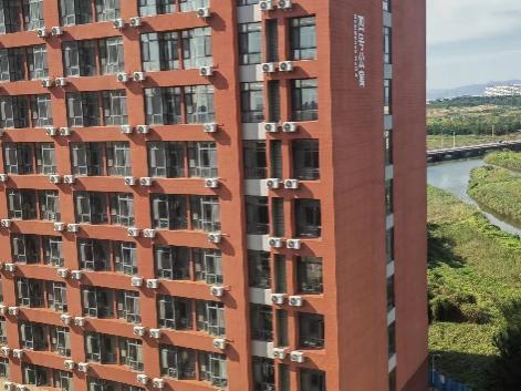
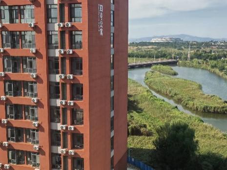
Figure 1. Bright complex picture group (Photo/Picture credit : Original)

Figure 2. Bright and simple picture group (Photo/Picture credit : Original)

Figure 3. Dim complex picture group (Photo/Picture credit : Original)

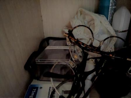
Figure 4. Dim simple picture group (Photo/Picture credit : Original)

4.2. Results

The second group screened outliers for display (Figure 5):

Figure 5. The second group of comparison, from top to bottom are RANSAC, least square, LMedS algorithm (Photo/Picture credit : Original)

4.3. Result analysis and discussion

Lowe's ratio testratio_thresh = 0.6 is set when FLANN algorithm is used for feature point screening. In order to unify variables, the threshold of RANSAC algorithm and LMedS algorithm is set to 6, and the least square method cannot set the threshold. The reprojection error in the experimental data can reflect the robustness of the algorithm. The larger the error, the lower the robustness (Table 6).

Table 6. Algorithm comparison in bright and complex case

In the bright and complex first environment, the reprojection errors of the different algorithms are arranged as follows: RANSAC< LMedS< Least square, so their robust arrangements can also be obtained: RANSAC> LMedS> Least square. At the same time, the experiment also measured the running time of each algorithm, which is arranged as follows: LMedS > Least square Least square > RANSAC. In summary, RANSAC's robustness and operating efficiency are superior to the other two algorithms in bright and complex environments. RANSAC is the environment of choice because it can process data sets containing outliers more efficiently and in less time.

Table 7. Algorithm comparison in bright and simple case:

When encountering a bright and simple environment, the reprojection error shown in the experiment is as follows: RANSAC< LMedS< Least square, and the corresponding robustness is as follows: RANSAC> LMedS> Least square. the running time tested by each algorithm in order from small to large is: Least square < RANSAC < LMedS. In contrast, RANSAC is also the most suitable algorithm for screening in bright and simple environments, which can be described as the optimal algorithm in bright environments (Table 7).

Table 8. Algorithm comparison in dim and simple case

Due to the dark and complex environment, the reprojection error and running time become much larger, and the reprojection error arrangement of the algorithm is shown: LMedS< RANSAC< Least square, so the robustness is: LMedS> RANSAC> Least square. and the running time ordering can also be obtained: Least square< LMedS< RANSAC. Although Least square algorithm has the shortest running time, its robustness is the worst, which will lead to a large error in the result, so in contrast, LMedS is more high-performance, if there are requirements for the running time, and there are not many outliers, it can try to use Least square algorithm, and finally, in the dim and complex case, LMedS has become the best algorithm (Table 8).

Table 9. Algorithm comparison in dim and complex cases

The last case is a dark and simple environment, and the experimental results in this environment are a little complicated. First, the gravity projection error is arranged as follows: RANSAC< LMedS< Least square, and then the robust ranking is obtained: RANSAC> LMedS> Least square. The running time will also be compared: RANSAC > LMedS> Least square (Table 9). RANSAC algorithms, although slower in terms of run time, are usually the best choice due to their superior performance in robustness, especially in the case of large noise and outliers. If running time is a critical factor when using the algorithm, and a high reprojection error is acceptable, the use of least squares may be considered. If these two kinds of performance are considered at the same time, the compromise LMedS algorithm can be chosen. In general, the RANSAC algorithm is the best solution, because the difference in time is not very large.

4.4. Experimental discussion summary

In this experiment, the experimental images are divided into four different situations, which are: bright complex environment, bright simple environment, dark complex environment, dark simple environment. The test is on the reprojection error (i.e., robustness) and runtime of each algorithm. During testing, RANSAC algorithm is the most robust in most environments, but it is less efficient in dim environments. In addition, LMedS is moderately superior in both robustness and efficiency in all cases, and is even better than RANSAC in dim and complex environments. At last, the efficiency of least squares algorithm is always high, but its robustness is relatively low, so the error of experimental results is large.

5. Conclusion

This paper discusses the performance of different algorithms in different environments by obtaining image database from mobile devices. The experimental environment includes bright complex environment, bright simple environment, dark complex environment and dark simple environment. The results show that RANSAC algorithm shows high robustness in most environments, but low efficiency in dim environments. The LMedS algorithm showed moderate superiority in all cases and was superior to RANSAC in dim and complex environments. In contrast, the least square algorithm always maintains a high efficiency, but its experimental results have a large error. In future investigations, researchers could consider using a combination of Least Squares to quickly obtain preliminary results, and then using RANSAC to further optimize and improve robustness, especially when working with more complex data sets.

References

[1]. DelSole, T., & Tippett, M. (2022). Linear Regression: Least Squares Estimation. In Statistical Methods for Climate Scientists (pp. 185–209). Cambridge University Press. https://doi.org/10.1017/9781108652078.010
[2]. Lowe, D. G. (2004). Distinctive Image Features from Scale-Invariant Keypoints. International Journal of Computer Vision, 60(2), 91-110. https://doi.org/10.1023/B:VISI.000 0029664.99615.94
[3]. Bay, H., Ess, A., Tuytelaars, T., & Van Gool, L. (2008). Speeded-Up Robust Features (SURF). Computer Vision and Image Understanding, 110(3), 346-359. https://doi.org/10.1016/j.cviu.2007.09.014
[4]. Verma, C. S., & Mon-Ju. (2009). Panoramic Image Mosaic. Retrieved from https://pages.cs.wisc.edu/~csverma/CS766_09/ImageMosaic/doc.pdf
[5]. Chen, Y., Wang, G., & Wu, L. (2019). Research on feature point matching algorithm improvement using depth prediction. The Journal of Engineering, 2019(23), 8905–8909. https://doi.org/10.1049/joe.2018.9142
[6]. Rublee, E., Rabaud, V., Konolige, K., & Bradski, G. (2011). ORB: An efficient alternative to SIFT or SURF. 2011 International Conference on Computer Vision (pp. 2564-2571). https://doi.org/10.1109/ICCV.2011.6126544
[7]. Meer, P., Mintz, D., Rosenfeld, A., & Kim, D. Y. (1991). Robust Regression Methods for Computer Vision: A Review. International Journal of Computer Vision, 6(1), 59-70.
[8]. Karami, E., Prasad, S., & Shehata, M. (2023). Image Matching Using SIFT, SURF, BRIEF and ORB: Performance Comparison for Distorted Images. https://arxiv.org/pdf/1710.02726
[9]. Suju, A., & Jose, H. (2017). FLANN: Fast approximate nearest neighbor search algorithm for elucidating human-wildlife conflicts in forest areas. 2017 International Conference on Signal Processing and Communication Networks (ICSCN) (pp. 1-6). https://doi.org/10.1109/ICSCN.2017.8085676
[10]. GeeksforGeeks. (2024). Least Square Method Definition graph and formula. Retrieved from https://www.geeksforgeeks.org/least-square-method/
[11]. Derpanis, K. G. (2010). Overview of the RANSAC Algorithm. Retrieved from http://www.cse.yorku.ca/~kosta/CompVis_Notes/ransac.pdf
Cite this article
Ren,Y. (2024). Performance Comparison of RANSAC and Other Model Estimation Methods in Panoramic Image Mosaic. Applied and Computational Engineering,105,82-90.
Data availability
The datasets used and/or analyzed during the current study will be available from the authors upon reasonable request.
Disclaimer/Publisher's Note
The statements, opinions and data contained in all publications are solely those of the individual author(s) and contributor(s) and not of EWA Publishing and/or the editor(s). EWA Publishing and/or the editor(s) disclaim responsibility for any injury to people or property resulting from any ideas, methods, instructions or products referred to in the content.
About volume
Volume title: Proceedings of CONF-MLA 2024 Workshop: Neural Computing and Applications
© 2024 by the author(s). Licensee EWA Publishing, Oxford, UK. This article is an open access article distributed under the terms and
conditions of the Creative Commons Attribution (CC BY) license. Authors who
publish this series agree to the following terms:
1. Authors retain copyright and grant the series right of first publication with the work simultaneously licensed under a Creative Commons
Attribution License that allows others to share the work with an acknowledgment of the work's authorship and initial publication in this
series.
2. Authors are able to enter into separate, additional contractual arrangements for the non-exclusive distribution of the series's published
version of the work (e.g., post it to an institutional repository or publish it in a book), with an acknowledgment of its initial
publication in this series.
3. Authors are permitted and encouraged to post their work online (e.g., in institutional repositories or on their website) prior to and
during the submission process, as it can lead to productive exchanges, as well as earlier and greater citation of published work (See
Open access policy for details).