1. Introduction

The factorization of large integers is a long-standing challenge in classical computing, and it underpins the security of widely utilized encryption methods, such as the RSA algorithm [1]. The classical difficulty of factoring large numbers ensures that RSA remains robust against conventional attacks. In 1994, Shor introduced a groundbreaking quantum algorithm that could factor large integers exponentially faster than any known classical algorithm, sparking significant interest in quantum cryptography and quantum computing [2]. Shor's algorithm, by harnessing quantum mechanics, posed a potential threat to RSA encryption by demonstrating an efficient means of factoring via quantum computation.

Since the inception of Shor's algorithm, researchers have made various attempts to enhance its efficiency, primarily aiming to reduce the number of quantum gates required. Despite this, substantial progress on Shor's original approach has proven elusive over the years. The problem of factoring large integers is thought to be hard classically. This difficulty establishes the basis of the RSA encryption algorithm [1]. In 1994, Shor published his famous quantum factoring algorithm, establishing an exponential speedup over classical methods. Over the years, there had been multiple attempts to improve and optimise Shor’s algorithm, for example trying to reduce the total number of quantum gates required. When the number to be factorised is an n-bit number N, the original Shor’s algorithm uses \( O(n^{2}\log{n}) \) quantum gates. Despite previous efforts, no one had managed to cut this down by a polynomial factor. This provides the first substantial speedup in nearly 30 years. \( O(n^{2}\log{n}) \)

To design good quantum algorithms, a lot of factors need to be considered. As a newly established result, a lot of improvements could be made on Regev’s factoring algorithm [2]. For example, Regev’s circuit required \( O(n^{\frac{3}{2}}) \) \( O(n^{\frac{3}{2}}) \) qubits, an increase from the 𝑂 𝑛 required in Shor’s; an unproven number theory assumption was also crucial in the argument. Several follow-up results have already surfaced, which include reducing the number of qubits, improving error tolerance, generalisations to other related problems and proving the number theory assumption in Regev’s original paper. This review article aims to give an overview of Regev’s factoring algorithm and its follow-up developments. This will be done in a way that is more accessible to people who are just getting into the field of quantum computing, or to researchers who are not familiar with these ideas. The hope is to push quantum computing forward by drawing more attention and effort. qubits, an increase from the \( O(n) \) \( O(n) \)

In the following, Shor’s factoring algorithm will be reviewed. An overview of Regev’s factoring algorithm is then given. Afterwards, the results in the two main follow-up papers, Ragavan and Vaikuntanathan, and Ekerå and Gärtner, are summarised. Finally, a discussion on existing knowledge and potential future developments are given.

This paper provides a comprehensive overview of Regev's recent contributions to quantum factoring, framed within the context of Shor's pioneering work. It presents an in-depth examination of Regev's methodology and its core innovations, such as the transition to higher-dimensional structures and the use of lattice-based techniques. Additionally, the paper highlights subsequent research developments, including improvements to qubit efficiency, error tolerance, and extensions of Regev's algorithm to related problems like discrete logarithms [5]. This review aims to offer accessible insights for new researchers and experts alike, fostering further exploration in the promising domain of quantum factoring algorithms.

2. Regev’s factoring algorithm

2.1. Review of shor’s factoring algorithm

The order-finding algorithm then then consists of two parts - the quantum procedure and the classical post-processing. The exponential speedup over classical methods is provided by the quantum procedure.

For the reduction to order-finding to work, there are two constraints [3]. Firstly, \( r \) \( r \) is asked to be even, or equivalently \( a = b^{2} mod N \) \( a = b^{2} mod N \) for some \( b \) \( b \) ; secondly, \( b^{r}∉ \{-1, 1\} mod N \) . The first condition implies \( (b^{r}-1)(b^{r}+1)=0modN \) , where the second condition then implies neither bracket is divisible by \( N \) \( N \) . Thus, the greatest common divisors \( \gcd{(N,b^{r}-1)} \) and gcd 𝑁, 𝑏 𝑟 +1 give non-trivial factors of 𝑁. For a uniformly chosen 𝑎, the two constraints are satisfied with good probability. By sampling different values of 𝑎, the reduction argument will work within a reasonable number of trials. and \( \gcd{(N,b^{r}+1)} \) give non-trivial factors of \( N \) \( N \) . For a uniformly chosen \( a \) \( a \) , the two constraints are satisfied with good probability. By sampling different values of \( a \) \( a \)

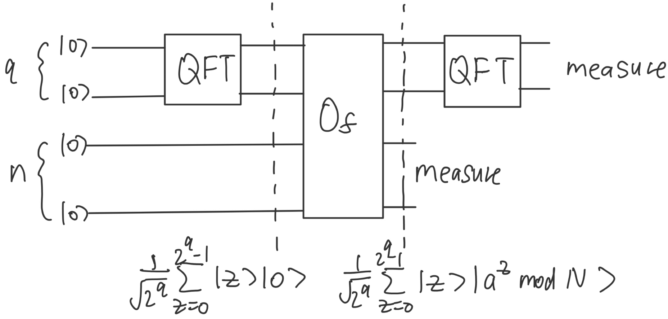
Figure 1. Quantum Circuit for Shor's Algorithm with Quantum Fourier Transform (QFT) (Photo credit: Original).

The order-finding problem is a case of the structure of the quantum procedure is similar to other famous quantum algorithms, such as Deutsch-Jozsa and Simon [4]. They all fall into the category of Hidden Subgroup Problems. Figure 1 shows a sketch for the quantum circuit of Shor's algorithm. For Shor's algorithm, the black-box has the ability to compute \( a^{z} mod N \) for any \( 1≤ z≤ N, \) a process called modular exponentiation. The quantum procedure can be broken into three parts. First, the first register is prepared in the state \( |0124*(010217*), \) then passed through a Hadamard gate to create the superposition state \( 2^{-n/2}\sum_{z=1}^{2^{n}-1} |z124*(z10217*) \) . Next, with the second register set to \( |0124*(010217*), \) the two registers are passed through the black-box; this stores the result of \( a^{z} mod N \) into the second register, resulting in the state \( 2^{-n/2}\sum_{z=1}^{2^{n}-1} |z124*(z10217*)|a^{z}modN124*(a^{z}modN10217*) \) . Finally, QFT is applied to the first register, after which the first register is measured.

The quantum procedure outputs (after dividing by \( N \) \( N \) ) an estimation to \( c/r \) \( c/r \) , where \( c \) \( c \) is a random number in \( 0,1,⋯,r-1 \) determined by the measurement process at the end. When the estimation is close enough to \( c/r \) \( c/r \) , the Continued Fraction Algorithm can be used to recover \( c/r \) \( c/r \) from the estimation. Note that this is the classical-post processing - computations are done classically rather than quantumly [5]. At the end, the order \( r \) can be retrieved from 𝑐/𝑟 provided 𝑐 is coprime to 𝑟. The two requirements that the estimation is accurate enough, and that 𝑐 is coprime to 𝑟, can be shown to happen with good probability. \( r \) can be retrieved from \( c/r \) \( c/r \) provided \( c \) \( c \) is coprime to \( r \) \( r \) . The two requirements that the estimation is accurate enough, and that \( c \) \( c \) is coprime to \( r \) \( r \)

Since building quantum devices is much harder than building classical computers, the priority is to try to reduce the amount of quantum resources needed. Of course, this is no use if the classical post-processing part cannot be done efficiently; this is not an issue in the case of the Continued Fraction Algorithm. The black-box is where the \( O(n^{2}\log{n}) \) gates in Shor's algorithm comes from. Modular exponentiation is typically done via repeated squaring, outlined below: \( O(n^{2}\log{n}) \)

Set the register to \( 1 \) .

Write the exponent \( z \) \( z \) in binary, 𝑧 1 𝑧 2 … 𝑧 𝑛 . in binary, \( z_{1}z_{2}… z_{n}. \)

For each \( j \) \( j \) from \( 1 \) to 𝑛, do: to \( n \) \( n \)

(i). Square the register;

(ii). If \( z_{j} = 1 \) , multiply the register by \( a \) \( a \) ; do nothing if 𝑧 𝑗 = 0. ; do nothing if \( z_{j} = 0. \)

In general, all intermediate results need to be stored using \( n \) \( n \) bits; therefore, this process involves \( O(n) \) \( O(n) \) multiplications between \( n \) -bit integers. Using fast multiplication, each multiplication costs 𝑂 𝑛 log 𝑛 gates, giving 𝑂 𝑛 2 log 𝑛 gates in total. \( n \) -bit integers. Using fast multiplication, each multiplication costs \( O(n\log{n}) \) \( O(n\log{n}) \) gates, giving \( O(n^{2}\log{n}) \) \( O(n^{2}\log{n}) \)

2.2. Overview of regev’s factoring algorithm

To reduce the number of gates used in the black-box, Regev applied two key ideas: moving to higher dimensions and keeping the numbers stored small.

Firstly, Shor's algorithm is simply generalised to having multiple variables. Instead of choosing one number \( a = b^{2} mod N, \) \( a = b^{2} mod N, \) Regev chose \( d \) \( d \) numbers \( a_{1}, a_{2}, …, a_{d} \) with \( a_{i} = b_{i}^{2} mod N. \) The black-box is generalised to compute 𝑖=1 𝑑 𝑎 𝑖 𝑧 𝑖 mod 𝑁 for 𝑧∈ ℤ 𝑑 . This is done via repeated squaring again: The black-box is generalised to compute \( \prod_{i=1}^{d} a_{i}^{z_{i}} mod N \) for \( z∈Z^{d} \) \( z∈Z^{d} \)

Set the register to \( 1, \)

For each exponent \( z_{i}, \) Write \( z_{i} \) in binary, \( z_{i1} z_{i2}… z_{in} \) .

For each \( j \) \( j \) from \( 1 \) to 𝑛, do: to \( n \) \( n \)

Square the register;

Compute \( \prod_{i=1}^{d} a_{i}^{z_{ij}} mod N \) ;

Multiply the register by \( \prod_{i=1}^{d} a_{i}^{z_{ij}} mod N \) .

He then worked in multi-dimensional structures called lattices. Lattice is a mathematical concept that already had wide applications in classical computing like lattice cryptography. Regev defined the two lattices [6]:

\( L={(z_{1},z_{2},…,z_{d})∈Z^{d}∣\prod_{i=1}^{d} a_{i}^{z_{i}}=1 mod N} \) (1)

\( L_{0}={(z_{1},z_{2},…,z_{d})∈Z^{d}∣\prod_{i=1}^{d} b_{i}^{z_{i}}∈{-1,1} mod N} \) (2)

Figure 2 visualises one possibility for the two lattices in the case \( d=2 \) \( d=2 \) . Throughout this section, it is very helpful to try the case \( d=1 \) , which often directly corresponds to Shor's algorithm. Table 1 compares various aspects of Regev's algorithm to Shor's algorithm. In this way, Regev reduced the factoring problem to a problem of finding elements in ℒ∖ ℒ 0 . \( d=1 \) , which often directly corresponds to Shor's algorithm. Table 1 compares various aspects of Regev's algorithm to Shor's algorithm. In this way, Regev reduced the factoring problem to a problem of finding elements in \( L∖ L_{0} \)

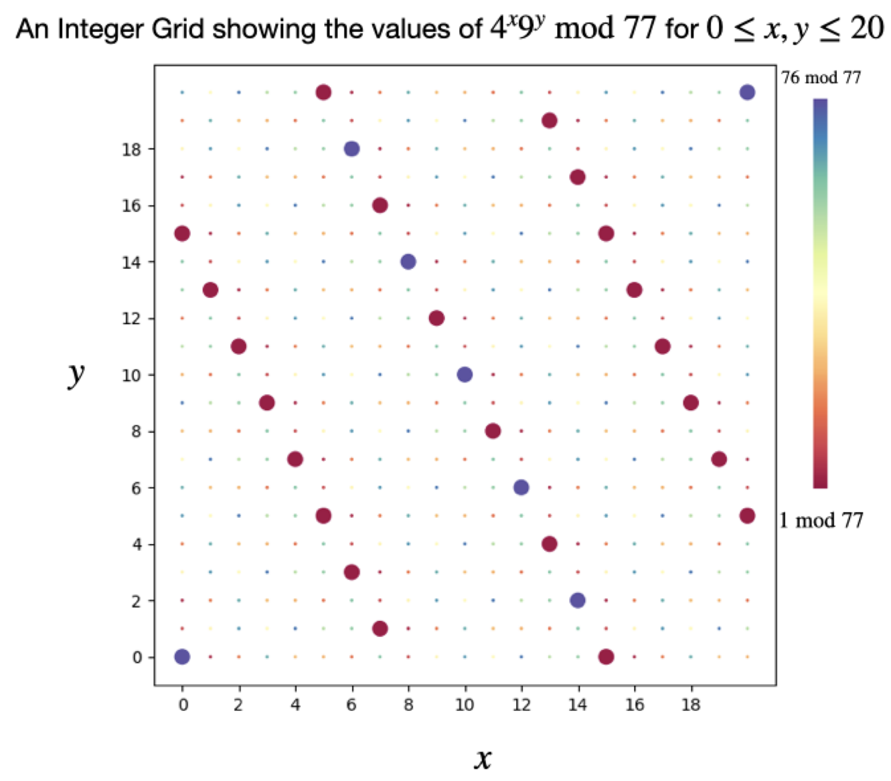
Figure 2. Modular Arithmetic Visualization (Photo credit: Original).

Table 1. A table comparing various aspects of Shor's algorithm and Regev's algorithm.

Figure 2 demonstrates this in two dimensions. In fact, a pigeon-hole argument shows that there exist a non-zero vector \( z∈L \) \( z∈L \) with \( |z_{i}|≤ 2^{\frac{n}{d}}. \) Fewer squaring operations are required to get to this exponent, which reduces the number of squaring operations in the black-box [7]. For Regev’s argument, the exponents actually have to go up to \( D \) , a number greater than 2 𝑛 𝑑 . \( D \) , a number greater than \( 2^{\frac{n}{d}}. \)

However, the total number of multiplications remains \( O(n). \) \( O(n). \) The products \( \prod_{i=1}^{d} a_{i}^{z_{ij}} mod N \) require in general \( d \) multiplications, which is a factor not present in Shor's algorithm (the case 𝑑=1). \( d \) multiplications, which is a factor not present in Shor's algorithm (the case \( d=1 \) \( d=1 \)

Fortunately, Regev's second ingredient does the trick. In Shor's algorithm, the number \( a \) \( a \) was chosen randomly. However, in Regev's algorithm, the numbers \( b_{i} \) (and so \( a_{i} \) ) were deliberately chosen to be fixed small numbers, more precisely \( O(\log{d}) \) \( O(\log{d}) \) -bit integers. The idea is that while the total number of multiplications was not reduced, the number of gates can be reduced by distributing and reordering the multiplications, in a way that maximises the number of small-number multiplications. Using a binary tree method, the products \( \prod_{i=1}^{d} a_{i}^{z_{ij}} mod N \) can be computed by only \( O(dlog^{3}d) \) gates. As explained later, choosing 𝑑= 𝑛 turns out to be optimal. In this way, Regev managed to construct a black-box using only 𝑂 𝑛 3/2 log 𝑛 gates. \( O(dlog^{3}d) \) gates. As explained later, choosing \( d=\sqrt[]{n} \) \( d=\sqrt[]{n} \) turns out to be optimal. In this way, Regev managed to construct a black-box using only \( O(n^{3/2}\log{n}) \) \( O(n^{3/2}\log{n}) \)

However, asking \( b_{i} \) to be small came at a cost. Although it was shown that there are vectors in \( L \) of norm at most \( 2^{O(n/d)} \) , they are not necessarily helpful for factoring. Recall that the reduction argument works for only vectors in \( L∖ L_{0} \) . Regev had to rely on a number theory assumption: that there exists a vector in \( L∖ L_{0} \) of norm at most \( T=2^{O(n/d)}. \) This is true if the numbers \( b_{i} \) were sampled uniformly instead of asked to be small.

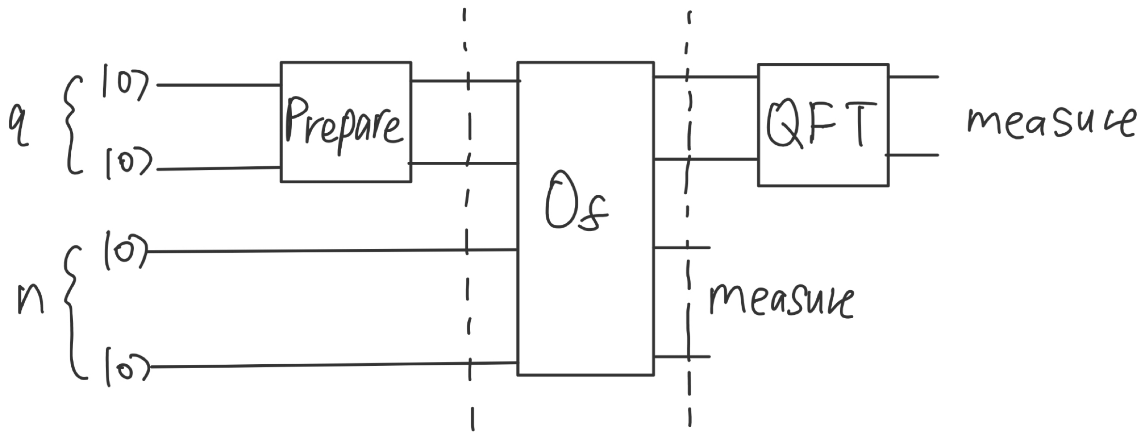
Figure 3. Quantum Circuit for Shor’s Algorithm with State Preparation and Quantum Fourier Transform (QFT) (Photo credit: Original).

Provided the assumption holds, Regev's algorithm works unconditionally, with fewer gates in the black-box compared to Shor's. The quantum procedure in Regev's algorithm is now described. The overall structure of the quantum procedure is very similar to Shor's, as shown in Figure 3. However, the specific implementations are more sophisticated due to the added dimensions.

(INSERT equation for Gaussian). Discrete Gaussian distributions already had applications in classical lattice problems before Regev's paper, see for example [8, 9]. Importantly, Gaussian distributions are computationally nice, for example the Fourier transform of a Gaussian distribution is (up to a multiplicative constant) Gaussian. These properties heavily simplified the calculations in Regev’s proofs.

After the improved black-box, a multi-dimensional version of QFT is applied to the first register. Formally, the dual lattice for a given lattice \( L \) is defined as

\( L^{*}={w∈R^{d}∣∀z∈L,10216*(w,z10217*)∈Z} \) (3)

Which is another lattice of the same dimension. Table 1 highlights how Shor's algorithm gives a demonstration of the dual lattice in the case \( d=1 \) \( d=1 \) . The element from ℒ ∗ is chosen uniformly from a list of possibilities, just as in the case of Shor's. . The element from \( L^{*} \)

The classical post-processing is then responsible for recovering an element in \( L∖ L_{0} \) from the estimation to \( L^{*} \) . This requires a more sophisticated argument than in the case of Shor's. Firstly, the entire quantum procedure is repeated \( d+4 \) \( d+4 \) times. To be able to gain enough information about \( L^{*} \) , at least \( d \) \( d \) runs of the quantum procedure is needed as \( L^{*} \) is \( d \) \( d \) -dimensional. Since the elements from \( L^{*} \) are chosen randomly, there are an additional 4 runs to make sure the entire lattice can be generated with probability at least 1/2. This gives a noisy sample of the dual lattice. Secondly, by cleverly constructing a new lattice ℒ ′ , Regev was able to recover certain vectors in the original lattice from the noisy sample of the dual lattice. are chosen randomly, there are an additional \( 4 \) runs to make sure the entire lattice can be generated with probability at least \( 1/2 \) . This gives a noisy sample of the dual lattice. Secondly, by cleverly constructing a new lattice \( L^{'} \)

This is thought to be hard, however the LLL algorithm provides a way to approximate the length of the shortest vector. When the lattice is \( d \) \( d \) -dimensional, this length is approximated to within a factor of \( 2^{d} \) . This agrees with the intuition that it is harder to recover information from higher-dimensional lattices. Thus, while having more dimensions seemingly improves the black-box by only contributing a factor of \( 2^{\frac{n}{d}} \) , the advantage starts to fade for large \( d \) \( d \) due to the factor of 2 𝑑 . This effectively fixes the optimal choice 𝑑= 𝑛 . due to the factor of \( 2^{d} \) . This effectively fixes the optimal choice \( d= \sqrt[]{n} \) \( d= \sqrt[]{n} \)

By applying the LLL algorithm (runs in polynomial time) in place of the Continued Fraction Algorithm, the classical post-processing is able to recover a short vector from \( L∖ L_{0} \) , which can then be used to factor \( N \) . \( N \)

Like in Shor's algorithm, several steps in Regev's algorithm are not guaranteed to work. However, overall the algorithm fails with bounded probability, and it is easy to check whether the algorithm has succeeded.

2.3. Discussion

This section contains several remarks.

However, having only \( O(n^{\frac{3}{2}}\log{n}) \) \( O(n^{\frac{3}{2}}\log{n}) \) gates in each run of the circuit is better for several reasons. Importantly, we expect quantum error correction to work better for smaller circuits, and that fewer errors would occur. On the other hand, the 𝑛 +4 repetitions can be run in parallel, saving overall runtime. gates in each run of the circuit is better for several reasons. Importantly, we expect quantum error correction to work better for smaller circuits, and that fewer errors would occur. On the other hand, the \( (\sqrt[]{n}+4) \)

Secondly, the total number of qubits used in Regev's algorithm was \( O(n^{\frac{3}{2}}) \) \( O(n^{\frac{3}{2}}) \) - for Shor's it was only 𝑂 𝑛 [10]. Fortunately, this has been reduced by Ragavan and Vaikuntanathan, making practical implementations of Regev's algorithm much more likely [11]. Ragavan and Vaikuntanathan also modified the classical post-processing part to make it more noise-robust [12]. - for Shor's it was only \( O(n) \) \( O(n) \)

Altogether, it must be said that the analysis was asymptotic. Hidden constants like the constant \( C \) \( C \) in 𝑅= 2 𝐶 𝑛 can make Regev's algorithm less effective for factoring small numbers. in \( R=2^{C\sqrt[]{n}} \) \( R=2^{C\sqrt[]{n}} \)

One potential investigation is to replace the Gaussian superposition with a uniform superposition, reverting to Shor's approach.

In 2024, Pilatte managed to prove the number theory assumption for a modified version of Regev's algorithm. In the proof, he used a less restrictive bound on the numbers \( b_{i} \) . This was not ideal for practical applications, as the increased size in \( b_{i} \) also increased the circuit size. For Regev's algorithm to be both unconditionally correct and practical, a proof for a stronger result is needed.

Lastly, Regev's factoring algorithm was extended to other related problems like discrete logarithm, by Ekerå and Gärtner [13].

3. Further developments

3.1. Reducing the number of qubits

To analyze the number of qubits used in a quantum circuit, often one starts from the corresponding classical circuit. The key characteristics in quantum computing is that computations are reversible, something not required for classical circuits. To convert a classical circuit with \( G \) \( G \) gates and 𝑆 bits into a quantum one, irreversible gates are replaced with reversible ones, and ancilla qubits are added to keep information around. The details can be found in [14]. gates and \( S \) \( S \)

The problem with Regev’s circuit originates from the black-box yet again. The first register uses \( \log{D^{\sqrt[]{n}}=O(n)} \) qubits and the second register uses \( n \) \( n \) qubits; each fast multiplication circuit uses \( O(n\log{n}) \) \( O(n\log{n}) \) ancilla qubits. This apparently results in \( O(n\log{n}) \) \( O(n\log{n}) \) qubits. Unfortunately, while modular multiplication can be done in-place, modular squaring cannot. Here, in-place means that the outcome of the operation is stored in the input register, whereas out-of-place means storing the outcome in a new register. It is difficult to make modular squaring reversible and in-place. The square root of a number modulo \( N \) is not necessarily unique, and to find even one of them is hard. Thus, for each squaring operation done in the black-box, the result needs to be stored in a separate register. Since there are 𝑂 𝑛 squaring operations and each result occupies 𝑂 𝑛 qubits, at least 𝑂 𝑛 3 2 qubits are needed. \( N \) is not necessarily unique, and to find even one of them is hard. Thus, for each squaring operation done in the black-box, the result needs to be stored in a separate register. Since there are \( O(\sqrt[]{n}) \) \( O(\sqrt[]{n}) \) squaring operations and each result occupies \( O(n) \) \( O(n) \) qubits, at least \( O(n^{\frac{3}{2}}) \) \( O(n^{\frac{3}{2}}) \)

To avoid this, Ragavan and Vaikuntanathan exploited the fact that in-place, reversible modular multiplications are easier to implement than modular squaring [15]. The idea is to use Fibonacci numbers instead of the powers of 2, something that appeared in the work of Kaliski [16]. In the following, every state is reduced modulo \( N \) \( N \) , so the notation is omitted. To start, two registers are initialised to \( |a124*(a10217*)|a124*(a10217*). \) Afterwards, repeatedly multiply the two registers together and store the result in the appropriate register. An example run would be \( |a124*(a10217*)|a124*(a10217*)↦ |a^{2}124*(a^{2}10217*)|a124*(a10217*)↦ |a^{2}124*(a^{2}10217*)|a^{3}124*(a^{3}10217*)↦ |a^{5}124*(a^{5}10217*)|a^{3}124*(a^{3}10217*) \) . This generates the Fibonacci sequence, which grows slightly slower than the powers of \( 2 \) , but still gets to the desired power of 𝑎 very efficiently. At the expense of an additional register, all squaring operations have been converted to multiplications. , but still gets to the desired power of \( a \) \( a \)

It can be proven by induction that every positive integer has such a decomposition, which can be easily found by a greedy algorithm: repeatedly finding the largest Fibonacci number smaller than the current number, then subtracting off this Fibonacci number from the current number. This decomposition can be written as \( z_{i}= \sum_{j=1}^{K} z_{ij}F_{j} \) , where \( z_{ij}∈-1,1 \) , \( F_{j} \) is the \( j \) \( j \) th Fibonacci number, and \( K \) \( K \) is the largest such that 𝐹 𝐾 ≤𝐷. By using Binet’s formula, it can be shown that 𝐾=𝑂 𝑛 . is the largest such that \( F_{K}≤D. \) By using Binet’s formula, it can be shown that \( K=O(\sqrt[]{n}) \) \( K=O(\sqrt[]{n}) \)

This decomposition is used to compute \( \prod_{i=1}^{d} a_{i}^{z_{i}} mod N \) :

\( \prod_{i=1}^{d} a_{i}^{z_{i}}= \prod_{i=1}^{d} \prod_{j=1}^{K} a_{i}^{z_{ij}F_{j}}= \prod_{j=1}^{K} (\prod_{i=1}^{d} a_{i}^{z_{ij}})^{F_{j}}=\prod_{j=1}^{K} c_{j}^{F_{j}} \) (4)

Defining the numbers \( c_{j} \) . Note that each \( c_{j} \) can be computed exactly as in Regev’s original algorithm, the only difference being the individual \( z_{ij} \) might not agree. This means the small numbers \( a_{i} \) can again be exploited to compute each \( c_{j} \) efficiently. The whole product can then be computed using the idea of Fibonacci exponentiation.

By analysing other multiplication algorithms, the number of qubits can be further reduced to \( O(n), \) though at the expense of having more gates. \( O(n), \)

3.2. Results on noise tolerance

For Regev’s original algorithm, all \( \sqrt[]{n}+4 \) runs of the quantum procedure need to be successful for the classical post-processing. This is not ideal in practice as quantum systems are exposed to noise from the environment, making some or all samples corrupted. Ragavan and Vaikuntanathan also managed to improve on noise-tolerance by showing that under certain assumptions on the noise, a modified version of Regev’s classical post-processing can work even when a fraction of the sample is corrupted. This involves running an algorithm that filters out the corrupted samples.

By definition, if \( v_{i} \) is in the dual lattice, then \( 10216*(u,v_{i}10217*) \) is an integer for any vector \( u \) \( u \) in the lattice. A key idea in Regev’s classical post-processing was that for any \( u \) \( u \) not in the lattice, then one can expect that there is some \( v_{i} \) in the dual lattice such that 𝑢, 𝑣 𝑖 is not close to any integer. This gives the ability to recognise which vectors 𝑢 are in the lattice and which are not. in the dual lattice such that \( 10216*(u,v_{i}10217*) \) is not close to any integer. This gives the ability to recognise which vectors \( u \) \( u \)

Assume for simplicity that now there is an error in the form of a uniformly chosen vector in \( [0,1]^{d} \) , which occurs with probability \( p \) \( p \) . The key idea is that if all the samples \( v_{i} \) from the dual lattice are not corrupted, then by a pigeon-hole argument, a small-number linear combination of these vectors gives a vector in \( Z^{d} \) . This implies that the linear combination of the noisy samples \( w_{i} \) gives a vector close to \( Z^{d} \) . However, even one corrupted sample would mean that any linear combination of the samples is uniformly distributed in \( [0,1]^{d}, \) and thus unlikely to be close to ℤ 𝑑 . Ragavan and Vaikuntanathan generalised the case of uniformly distributed error by intuitively abstracting the property that the error distribution is ‘well-spread’ with respect to the lattice. This gave a way to detect corrupted samples under a mild assumption on the error distribution. and thus unlikely to be close to \( Z^{d}. \)

Regev used the fact that \( \sqrt[]{n}+4 \) samples of the dual lattice are enough to generate it with probability at least \( 1/2 \) . The case of Ragavan and Vaikuntanathan is different, since they first obtained \( α\sqrt[]{n} \) \( α\sqrt[]{n} \) samples from the quantum procedure, for some \( α>1, \) \( α>1, \) then selected a subset of \( γd \) \( γd \) samples, which are assumed to be uncorrupted by running the error detection algorithm. Thus, a stronger version of the fact was applied – that provided \( γ \) \( γ \) is close enough to \( α \) , any such subset of 𝛾𝑑 samples generate the dual lattice with probability at least 1/2. Finally, by assuming the error probability 𝑝 is small enough, there are likely enough uncorrupted samples to make up a subset of 𝛾𝑑, completing the argument. Once the subset of uncorrupted samples is obtained, Regev’s classical post-processing can be applied with little modifications – the central argument is still running LLL to obtain a short basis for the original lattice. \( α \) , any such subset of \( γd \) \( γd \) samples generate the dual lattice with probability at least \( 1/2 \) . Finally, by assuming the error probability \( p \) \( p \) is small enough, there are likely enough uncorrupted samples to make up a subset of \( γd, \) \( γd, \)

Independently, Ekerå and Gärtner also discussed error-robustness of Regev’s algorithm. However, this relied on assumptions on the structure of the lattice and the error distribution, in particular the number theory assumption that the lattice \( L \) has a short basis, which is stronger than Regev’s number theory assumption. As commented by Ragavan and Vaikuntanathan, this should be seen as a distinct contribution to noise-tolerance of Regev’s algorithm.

3.3. Extension to discrete logarithm

Like order-finding, this problem can be state in general groups. For simplicity, only the version in \( Z_{p}^{*}=1,⋯,p-1 \) is stated here: given \( g∈Z_{p}^{*} \) \( g∈Z_{p}^{*} \) and \( x=g^{e} \) \( x=g^{e} \) for some unknown \( e \) \( e \) , determine 𝑒= log g 𝑥 . Note that 𝑟 - the order of 𝑔 - is assumed to be known, which can be found by first running the order-finding quantum algorithm. , determine \( e=\log_{g}{x}. \) \( e=\log_{g}{x}. \) Note that \( r \) \( r \) - the order of \( g \) \( g \)

Shor’s approach was to essentially apply the two copies of order-finding circuit to two separate registers, one responsible for exponentiating \( g \) \( g \) and the other responsible for exponentiating \( x \) \( x \) . For two integers \( a \) \( a \) and \( b \) \( b \) , the black-box computes 𝑔 𝑎 𝑥 𝑏 mod 𝑁 and stores the result in a third register. At the end, QFT is applied to each of the first two registers, then the results are measured. This obtains two approximations, one to 𝑐/𝑟 and one to 𝑒𝑐/𝑟. The Continued Fraction Algorithm can then be applied to recover these two fractions, after which 𝑒 can be found. , the black-box computes \( g^{a}x^{b} mod N \) and stores the result in a third register. At the end, QFT is applied to each of the first two registers, then the results are measured. This obtains two approximations, one to \( c/r \) \( c/r \) and one to \( ec/r \) \( ec/r \) . The Continued Fraction Algorithm can then be applied to recover these two fractions, after which \( e \) \( e \)

There were two approaches, one with pre-computation and one without. The one without pre-computations (other than finding \( r) \) is presented here. \( r) \)

To be able to exponentiate \( x \) \( x \) and \( g \) , which are not necessarily small, the small-number restriction in Regev’s algorithm must be relaxed a bit. Notice that not all number 𝑏 𝑖 need to be small – there can be a constant number of them being large, without affecting the asymptotic size of the circuit. Thus, Ekerå and Gärtner proposed to look at the lattice \( g \) , which are not necessarily small, the small-number restriction in Regev’s algorithm must be relaxed a bit. Notice that not all number \( b_{i} \)

\( L_{x, g}={(z_{1},z_{2},…,z_{d})∈Z^{d}∣x^{z_{d-1}}g^{z_{d}}\prod_{i=1}^{d-2} a_{i}^{z_{i}}=1 mod N} \) (5)

Where \( a_{i} \) are \( O(\log{d}) \) \( O(\log{d}) \) -bit integers as before. The black-box then computes this new product modulo \( N \) \( N \) , where the product of \( a_{i} \) can be computed efficiently as in Regev’s algorithm, and x z d−1 and g z d are computed using the typical repeated squaring. The number of qubits is also subject to the optimisation of Ragavan and Vaikuntanathan. can be computed efficiently as in Regev’s algorithm, and \( x^{z_{d-1}} \) and \( g^{z_{d}} \)

Fortunately, a version of the assumption has been proven by Pilatte, again under the relaxation that \( a_{i} \) are slightly larger numbers. Under this assumption, the number \( e \) \( e \) can then be retrieved. The quantum procedure and classical post-processing work the same as in Regev’s algorithm. Using the LLL algorithm, a short basis for \( L_{x, g} \) can be recovered. Finally, this basis can be used to find \( (0, …,0, 1, -e)∈ \) \( L_{x, g} \) and therefore 𝑒, which just follows from solving a linear system of equations. and therefore \( e \) \( e \)

The change of bases formula for logarithm can be exploited to further optimise the algorithm. By using e = \( \log_{g}{x} \) = \( \log_{g^{'}}{x}/\log_{g^{'}}{g} \) , the number \( g \) \( g \) can be replaced by a small number \( g^{'} \) , and \( \log_{g^{'}}{g} \) can be pre-computed. Less resources are then needed to compute log g ′ 𝑥 can be pre-computed. Less resources are then needed to compute \( \log_{g^{'}}{x} \)

4. Conclusion

This paper has provided a comprehensive overview of Regev's recent advancements in quantum factoring algorithms, building on Shor's foundational work. By introducing multi-dimensional structures and utilizing lattice-based techniques, Regev has significantly reduced the gate complexity for quantum factoring. This advancement represents a major step forward in quantum computing, offering potential efficiency improvements over Shor’s algorithm despite the increased qubit requirements and reliance on an unproven number theory assumption. In addition, recent developments by Ragavan and Vaikuntanathan, Ekerå and Gärtner, and Pilatte have further refined Regev's approach, focusing on reducing qubit counts, enhancing noise tolerance, and extending the algorithm to other problems, like discrete logarithms. These contributions collectively push the boundaries of quantum computing, making the practical implementation of quantum factoring more feasible. Looking ahead, several intriguing research directions remain. Future work could explore alternative initialization strategies, such as replacing the Gaussian superposition with uniform superpositions, to streamline the algorithm further. Additionally, improving the proof of Regev's number theory assumption for smaller numbers or finding ways to strengthen Pilatte’s results on correctness could bolster the algorithm’s practical utility. Exploring other optimizations for error tolerance and robustness will also be crucial as quantum hardware continues to evolve. By addressing these challenges, researchers can continue to refine Regev's algorithm, paving the way for broader applications and advancements in quantum cryptography and computation.

References

[1]. Aharonov D, Regev O 2005 Lattice Problems in NP coNP [online] Available: https://cims.nyu. edu/~regev/papers/cvpconp.pdf
[2]. Ekerå M, Gärtner J 2024 Extending Regev’s Factoring Algorithm to Compute Discrete Logarithms Post-Quantum Cryptography Springer Nature Switzerland pp 211–242 ISBN 9783031627460 DOI 10.1007/978-3-031-62746-0_10 [online] Available: http://dx.doi.org/10. 1007/978-3-031-62746-0_10
[3]. Kiebert M 2024 Oded Regev’s Quantum Factoring Algorithm [online] Available: https:// vdwetering.name/pdfs/thesis-midas.pdf
[4]. Nielsen MA, Chuang IL 2000 Quantum Computation and Quantum Information Cambridge University Press
[5]. Pilatte C 2024 Unconditional correctness of recent quantum algorithms for factoring and computing discrete logarithms [online] Available: https://arxiv.org/pdf/2404.16450v1
[6]. Ragavan S, Vaikuntanathan V 2024 Space-Efficient and Noise-Robust Quantum Factoring arXiv:2310.00899 [quant-ph] [online] Available: https://arxiv.org/abs/2310.00899
[7]. Regev O 2023 An Efficient Quantum Factoring Algorithm arXiv:2308.06572 [quant-ph] [online] Available: https://arxiv.org/abs/2308.06572
[8]. Regev O 2004 Lecture 2: LLL Algorithm [online] Available: https://cims.nyu.edu/~regev/ teaching/lattices_fall_2004/ln/lll.pdf
[9]. Kaye P, Laflamme R, Mosca M 2007 An Introduction to Quantum Computing Oxford University Press
[10]. Harvey D, van der Hoeven J 2021 Integer multiplication in time O(n log n) Annals of Mathematics 2(193) 563–617
[11]. Shor PW 1994 Algorithms for quantum computation: Discrete logarithms and factoring 35th Annual Symposium on Foundations of Computer Science Santa Fe, New Mexico, USA IEEE Computer Society pp 124–134
[12]. Pomerance C 2001 The expected number of random elements to generate a finite abelian group Periodica Mathematica Hungarica 43(1-2) 191–198
[13]. Zeckendorf E 1972 Representations of natural numbers by a sum of Fibonacci numbers and Lucas numbers Bulletin of the Royal Society of Sciences of Liege 179–182
[14]. Kaliski BS Jr 2017 Targeted Fibonacci exponentiation arXiv preprint arXiv:1711.02491
[15]. Acciaro V 1996 The probability of generating some common families of finite groups Utilitas Mathematica 243–254
[16]. Regev O 2024 Presentation at Simons Institute: An Efficient Quantum Factoring Algorithm — Quantum Colloquium [online] Available: https://www.youtube.com/watch?v=Uzn93GjAfRg)
Cite this article
Chen,R.L. (2024). An Overview of Regev’s Quantum Factoring Algorithm and Its Recent Developments. Applied and Computational Engineering,110,161-169.
Data availability
The datasets used and/or analyzed during the current study will be available from the authors upon reasonable request.
Disclaimer/Publisher's Note
The statements, opinions and data contained in all publications are solely those of the individual author(s) and contributor(s) and not of EWA Publishing and/or the editor(s). EWA Publishing and/or the editor(s) disclaim responsibility for any injury to people or property resulting from any ideas, methods, instructions or products referred to in the content.
About volume
Volume title: Proceedings of CONF-MLA 2024 Workshop: Securing the Future: Empowering Cyber Defense with Machine Learning and Deep Learning
© 2024 by the author(s). Licensee EWA Publishing, Oxford, UK. This article is an open access article distributed under the terms and
conditions of the Creative Commons Attribution (CC BY) license. Authors who
publish this series agree to the following terms:
1. Authors retain copyright and grant the series right of first publication with the work simultaneously licensed under a Creative Commons
Attribution License that allows others to share the work with an acknowledgment of the work's authorship and initial publication in this
series.
2. Authors are able to enter into separate, additional contractual arrangements for the non-exclusive distribution of the series's published
version of the work (e.g., post it to an institutional repository or publish it in a book), with an acknowledgment of its initial
publication in this series.
3. Authors are permitted and encouraged to post their work online (e.g., in institutional repositories or on their website) prior to and
during the submission process, as it can lead to productive exchanges, as well as earlier and greater citation of published work (See
Open access policy for details).