1. Introduction

With the development of The Times, for the pursuit of higher quality of life and higher technological development. Automated driving has become one of the important technologies to facilitate life. Research in the direction of automation has been carried out in the last century. In the 1939-40s, General Motors introduced the concept of autonomous driving at the New York World's Fair, laying the groundwork for future developments. The path planning algorithm must take into account various factors, including vehicle dimensions, parking space size and obstacle information to optimize the path from the current location to the target parking space [1]. Its primary objective is to determine a safe and efficient driving path for autonomous vehicles, allowing them to navigate the dynamic road and traffic conditions.

The main purpose of this study is to review current real-time path planning algorithms and evaluate their performance in dynamic environments.

This paper will start with the analysis of the A* algorithm and Dijkstra, then explore more excellent algorithms such as RRT and PRM in depth, use literature to provide data to verify the correctness of the results, and finally introduce an optimization method -MPC.

2. Five algorithm characteristics

Path planning is a fundamental aspect of robot application. It is very important to implement path planning in a dynamic environment. The most basic and widely used path planning algorithms are Dijkstra's algorithm and A* search algorithm.

2.1. Dijkstra algorithm

Dutch computer scientist Edsger W. Dijkstra proposed the Dijkstra algorithm in 1956. This algorithm is widely used to calculate the shortest path (non-negative weighting) in graphs. Dijkstra's algorithm starts at the source point and gradually expands to the whole graph. The shortest path of each node is determined step by step by greedy strategy. The greedy strategy can be understood as pursuing the minimum cost of the current step, regardless of the impact on the future. The algorithm obtains the global optimal solution through a series of local optimal choices. This process can be divided into three key steps: 1. Initialization: The estimated initialization is infinite to represent the unknown actual path. 2. Node selection: Use the greedy strategy to select the node with the shortest distance from the source point as the processing node. 3. Relaxation operation: Supposed to go from point A to point C, but there is point B between point A and point C. The distance from point A to point C is 10, the distance from AB is 3, and the distance from BC is 5. The path taken through ABC is 3+5=8. The ABC path is superior.

Dijkstra algorithm is mainly used in network routing and map software navigation system. During each iteration, it updates the path by selecting the node data closest to the start.

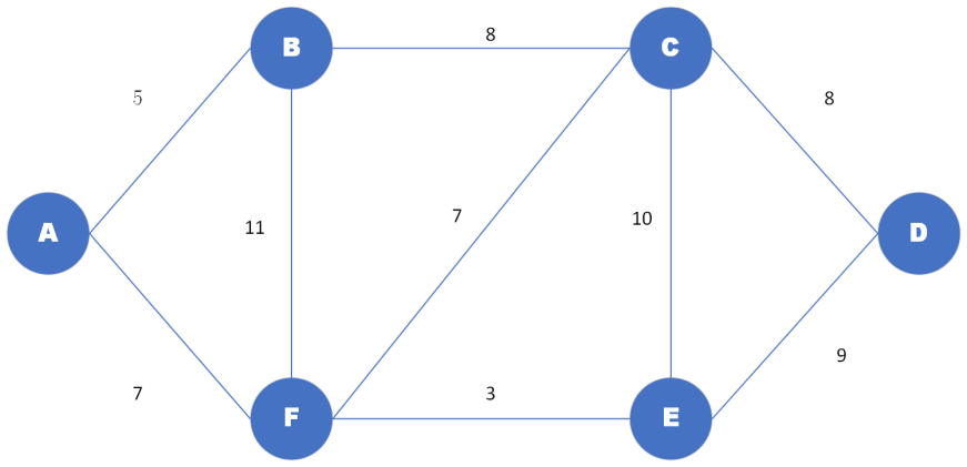
Figure 1. Simplified Dijkstra's algorithm sample graph

The data in the table represents the distance from the starting point a to the poi.

Dijkstra's shortest path is simplified as shown in the Figure 1 above. "()" in the table indicates the previous point connected to the point, and "__" in the table indicates that the data has been included. At first iteration, the distance between A and A is 0. At second iteration, the distance between node B and node F near node A is updated. Point B has the shortest distance from the starting point, which is 5. Therefore, B is included as the optimal path node. In the next iteration, try to update the nearest point of the newly marked node B. These are node F and node C. Suppose that the path from point A to B to C is the optimal path length of 13, which is less than infinity. Therefore, update the distance of node C. If this research look at node F, if the distance from A to B to F is 16. But this path is greater than the distance from node A to node F. So node F is not updated. Then the shortest path node F is found among all not-updated nodes and included in the optimal path node. In the fourth iteration, the adjacent points C and E of F are updated. The path of AFC is larger than the path of ABC, so the data at point C is not updated. AFE path distance is 10, node E is included as the optimal path node. In the next iteration, the nodes near E are C and D and D is the end point. The length of the AFED path is 19. Update the data at point D to 19. Because path ABC is superior to AFEC, the data at point C is not updated, and node C is included as the optimal node. In the sixth iteration, the adjacent points E and D of node C are detected. Don’t update point E and point D data. At this time, the algorithm is finished, and you can see that the shortest path in the Figure 2 is AFED. According to this simplified example, two rules can be found: 1. Each iteration selects the node closest to the starting point from the unmarked node for marking and includes it in the optimal path. 2. If the same node is reached, but the distance of the path explored later is shorter, the path will be updated to the optimal path to replace the previous data. Because it does not have to traverse the entire map like Dijkstra's algorithm, this algorithm can speed up the discovery of the shortest path [2].

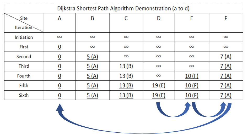
Figure 2. Verify Dijkstra's algorithm by backward inference

2.2. A-star algorithm

Dijkstra's algorithm was improved based on its shortcomings. The A-star was proposed by Peter Hart, Nils Nilsson and Bertram Raphael in 1968. A-star algorithm is a heuristic search algorithm, which is an optimization algorithm of Dijkstra's algorithm. Unlike Dijkstra's algorithm, which has to traverse the entire map. The A-star algorithm determines the optimal direction for path planning based on the estimated cost. In Figure 3, the two numbers added in the square represent the current cost (g(n)) and the estimated cost (h(n)) respectively. The current cost represents the total distance traveled from the starting point to the point. The estimated cost is not an exact value and can be estimated using methods such as Manhattan Distance or Euclidean Distance [3]. Where the Manhattan Distance means the sum of the vertical and horizontal Distances of two points when they can only move in the vertical or horizontal Direction. Euclidean Distance is the straight-line distance between two points. The Manhattan Distance is easy to calculate, so this research use the Manhattan Distance. Based on heuristic search, the a-star algorithm selects the least costly step for planning. It can be written as the expression f(n)=g(n)+h(n). From the results, a-star algorithm seems to have A "directional". As shown in Figure 4 figure 5, the algorithm will directionally select the node '1+3' closest to the end point as the optimal node for traversal. The A-star algorithm selects the direction with the smallest f (n) for path planning and repeats the execution.

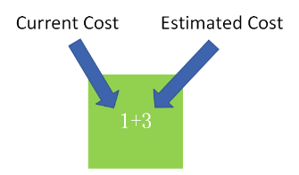
Figure 3. Block value definition

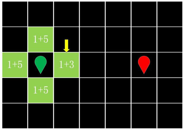
Figure 4. Optimal path node.

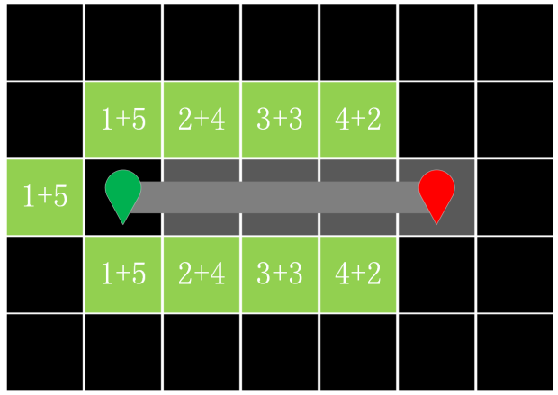
Figure 5. Optimal path

2.3. RRT algorithm

The Rapidly exploring Random Tree (RRT) algorithm is a sample-based path planning algorithm proposed by LaValle in 1998. The core of RRT is to use random sampling technology to randomly generate a tree structure extending from the starting point to the destination like Figure 6. The algorithm extends the search scope by randomly selecting nodes in the search space and connecting them with the existing tree structure. RRT has the ability to process high-dimensional space, and can generate a large quantity of random tree structures in a short time, which can quickly find a feasible path in a complex environment through connection. RRT is capable of handling complex and unknown Spaces containing random obstacles, as well as high and dynamic environments [4].

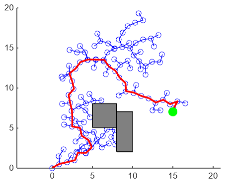
Figure 6. RRT algorithm run by MATLAB

2.4. PRM algorithm

The Probabilistic Roadmap Method (PRM) is an effective path planning technique that relies on constructing a probabilistic roadmap to facilitate pathfinding. The algorithm begins by randomly sampling multiple points within the search space, distributed across the free space of the environment. This sampling process does not depend on a detailed environmental model, making PRM adaptable to various complexities of the environment. Once the sampling points are generated in Figure 7, the algorithm constructs a graph by connecting these points based on certain connectivity conditions, such as creating edges between points within a specific distance to capture potential paths in the environment. During the graph construction, collision detection is performed to ensure that the connections between points do not intersect with obstacles. For pathfinding, PRM utilizes the constructed graph to search for a path from the start point to the goal, often employing algorithms like Dijkstra or A* for this purpose. Additionally, to enhance path quality and planning efficiency, PRM can optimize the graph by refining nodes and edges or adding more nodes to improve the smoothness and connectivity of the path. These characteristics make PRM particularly effective in static environments, especially for scenarios requiring global path planning.

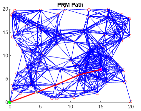
Figure 7. PRM algorithm run by MATLAB

2.5. MPC algorithm

Model Predictive control (MPC) is an advanced control strategy. It is widely used in dynamic systems, especially in the path planning of autonomous vehicles. The core principle of MPC involves predicting the future behavior of the system within a limited time frame and optimizing the control inputs accordingly. At each time step, the algorithm solves an optimization problem that minimizes the cost function, typically including provisions for tracking the desired trajectory and avoiding obstacles, while complying with system constraints. This makes MPC especially effective in generating viable and safe paths. For example, the MPC algorithm can not only plan the path of the vehicle, but also calculate the best acceleration, deceleration, and cornering strategies to enable the vehicle to navigate complex roads in the most efficient way. In Figure 8, the first graph is a vehicle location map, showing how the vehicle changes over time. Ideally, the vehicle will gradually approach the reference position. The second diagram is the control input diagram, which shows how the control inputs change over time. The control inputs can be acceleration and steering wheel Angle. This precise control makes MPC very effective in autonomous driving, especially in situations where precise control of vehicle movement is required, such as parking or navigating in urban environments. The predictive and iterative nature of the algorithm allows it to adapt to changing conditions in real time, making it indispensable in complex, dynamic scenarios that may not be possible with traditional methods. By adjusting the control inputs, the system is able to respond in real time to changing circumstances or demands, enabling the vehicle to travel accurately along a predetermined path. The MPC algorithm uses a predictive model to calculate a series of optimal control inputs to bring the output of the system as close to the target as possible. The algorithm performs well in handling constraints and optimization.

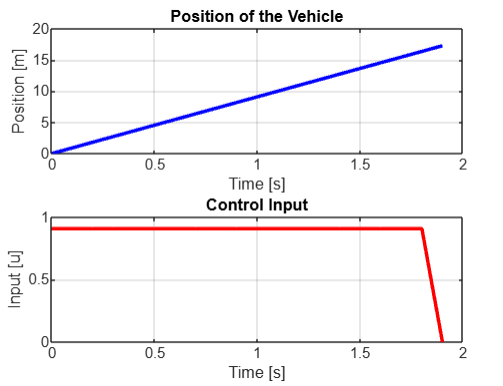
Figure 8. MPC algorithm running status

3. Discussion

The time complexity of an algorithm is often used to measure the efficiency of an algorithm in processing inputs of different sizes. It's denoted by O. In Dijkstra's algorithm, complexity is expressed as O((V+E) log v). “V” is the number of fixed points and “E” is the number of sides. According to the expression, the running time of Dijkstra algorithm is determined by the number of edges and vertices. This means that in some cases such as in densely distributed urban transportation networks, having more vertices and edges can lead to a significant increase in complexity. Dijkstra is an algorithm for finding a single source shortest path. At the same time, Dijkstra's algorithm has a flaw that is the weight of the edge cannot be negative. For example, in some economic models, edge weights may represent benefits or costs, and negative values may be used to represent losses. This is the limitation of D algorithm. Although the A-star algorithm is an improvement of Dijkstra's algorithm, the A-star algorithm also cannot handle negative-weighted edges. The A-star algorithm traverses fewer images than Dijkstra. This directional traversal saves events. Dijkstra's algorithm and a-star's algorithm have their own advantages and disadvantages. Dijkstra's algorithm needs to traverse more nodes to find the optimal path. When the information of other nodes is needed, it can be read directly. Therefore, it is more suitable for map navigation, providing users with the optimal path from the starting point to all nodes [3]. In contrast, although the A algorithm can display the shortest path more quickly, the generated path is usually composed of straight lines [4]. However, Dijkstra and A* algorithms have high computational complexity when handling large-scale or high-dimensional environments, which can lead to excessively long computation times, limiting their performance in real-time dynamic environments [6]. The complexity of a-star algorithm is O (b**d). "b" is the number of possible extensions per node. "d" is the shortest path length from the starting point to the destination node. This proves that the complexity of a-star algorithm is related to the number of nodes and the optimal path length. If you just use the greedy algorithm, something like Figure 9. However, both Dijkstra algorithm and a-star algorithm used the greedy strategy without hitting an obstacle and then changing the path. Dijkstra algorithm uses the greedy strategy to evaluate the actual path cost (cumulative weight) from the starting point to the current node. In each iteration, the shortest node found is selected for expansion. Dijkstra algorithm finds the shortest path for each node in this way. The greedy algorithm, on the other hand, only focuses on local information and selects the nearest node in each section. Therefore, the global optimal solution cannot be found. This makes Dijkstra algorithm more reliable than the greedy algorithm when solving the path problem. The a-star algorithm is more efficient than Dijkstra algorithm in figure10. In Dijkstra's algorithm, the cost of calculating the path from the starting point to the current node is g (n) in a-star's algorithm. The a-star algorithm also introduces the heuristic function h (n) [5]. This allows this algorithm to consider both the cost of the path traveled and the potential cost of reaching the target node [6][7]. This allows the a-star algorithm to avoid worthless exploration like the greedy algorithm and avoid falling into sub-optimal solutions.

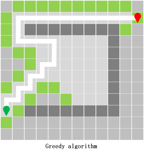
Figure 9. Greedy algorithm.

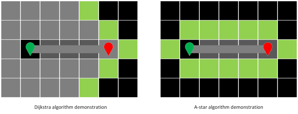
Figure 10. Algorithm comparison.

When evaluating the RRT algorithms and PRM algorithms, it is crucial to consider their differing strengths and how these advantages manifest in various scenarios. One key distinction is in their approach to exploring the environment. RRT excels in quickly navigating through high-dimensional spaces by dynamically expanding a tree structure. This allows RRT to efficiently handle dynamic or partially known environments where changes may occur unpredictably. In contrast, PRM is designed for static environments where a comprehensive roadmap can be precomputed. While PRM's roadmap provides a global view of the environment, making it easier to find smoother and more optimal paths, this advantage diminishes in dynamic settings where the environment might change after the roadmap is constructed. Another significant difference lies in path quality. PRM typically generates smoother and more optimal paths due to its reliance on a globally connected roadmap. This advantage makes PRM preferable in applications where the quality and smoothness of the path are paramount, such as in environments with narrow passages or when optimizing for energy efficiency. However, RRT often produces sub optimal and less smooth paths due to its random sampling nature, which may require post-processing to improve the path's quality. This is a trade-off for RRT ability to rapidly explore new areas without the need for extensive precomputation. When considering computational efficiency, RRT tends to be more efficient in scenarios where real-time processing is critical, as it does not require pre-building a roadmap. PRM, on the other hand, can be computationally expensive during the roadmap construction phase, especially in high-dimensional spaces. However, once the roadmap is built, PRM can find paths more efficiently than RRT, especially in complex environments with many obstacles. This difference makes PRM more suitable for applications where the environment is well-known and does not change frequently, while the strength lies of RRT in its adaptability and speed in dynamic settings. In summary, RRT offers greater flexibility and speed in environments where real-time adaptation is necessary, at the cost of path quality, while PRM provides higher quality paths and is more efficient in static environments but lacks the adaptability required for real-time changes. The choice between these two algorithms depends on the specific needs of the application, particularly regarding environmental stability and the importance of path smoothness and optimality. Table 2 compares and quantifies the capabilities of the five algorithms through the operation and experience of the algorithms. The PRM algorithm performs well in path planning in large-scale environments, especially for warehouse automation, robotic navigation, and logistics transportation, as it significantly reduces run time by randomly distributing points on a map and connecting them to form a viable path map [8].

Table 2. Five algorithms quantized comparison

4. Conclusion

The application of the current path planning algorithm in the autonomous driving technology needs to be considered from many angles, such as the calculation speed of the algorithm, the length of the each path planning and whether the solution conforms to the actual road conditions. When traversing the entire graph structure, Dijkstra's algorithm has significant advantages, especially for navigation scenarios where the shortest path needs to be found. It can not only show the shortest path, but also record the information of all traversing nodes, and quickly switch paths in case of obstacles or road closures. So it is more suitable for game development, robot navigation, and real-time path planning in dynamic environments. The A algorithm's real-time performance may be limited in a rapidly changing environment, especially when it needs to deal with complex dynamic changes. In addition, the A* algorithm also has high computational complexity when dealing with large-scale or complex environments. For RRT algorithms, although it may not be able to show the optimal path, due to it can find a path in narrow Spaces and avoid obstacles, it is very suitable for application in urban road design or robot navigation and autonomous driving in unstructured environments. However, the paths generated by RRT and PRM algorithms are often not smooth enough, and additional smoothing processing is required to improve the feasibility and comfort of the path. However, PRM does not perform as well as other algorithms when dealing with dynamic obstacles, and its adaptability to environmental changes is poor. In autonomous driving, MPC (Model Predictive Control) algorithm has a unique advantage. It can not only plan the path, but also calculate the optimal acceleration, deceleration and steering strategies during the planning process, so that the vehicle can be optimally driven on complex roads. This fine control makes MPC algorithms perform well in scenarios where precise control of vehicle movement is required, such as parking or driving on city roads. However, MPC algorithms also have some problems, such as high computational complexity, strong dependence on models, difficulty in solving optimization problems, lack of adaptability and robustness, and complex implementation, which may affect their performance in highly dynamic and uncertain environments.

To sum up, although each path planning algorithm has its unique advantages in different application scenarios, they also have their own limitations, especially in complex and dynamic environments, which limit their performance and efficiency in practical applications [9][10]. Therefore, when selecting a path planning algorithm suitable for automatic driving, it is necessary to comprehensively consider the computational efficiency, path smoothness, real-time performance, environmental adaptability, and safety of the algorithm to ensure its effectiveness and reliability in actual scenarios. Path planning algorithm has a wide range of practical significance. The performance of different algorithms in various complex environments varies greatly and finding the most suitable algorithm or combination to cope with the changing conditions on the actual road is the key to driving technological progress.

References

[1]. Han Z Sun H Huang J Xu J Tang Y Liu X 2024 Path Planning Algorithms for Smart Parking: Review and Prospects World Electric Vehicle Journal vol 15 no 7 pp322
[2]. Sun X Shen Y Zhang H 2024 A stable satellite routing algorithm based on a-star algorithm in dynamic networks Journal of Physics Conference Series
[3]. Elizabeth K Real-Time Graph-Based Path Planning for Autonomous Racecars. 2023 www.proquest.com/docview/2890800358/FA08369D35334CB4PQ/2?%20Theses&accountid=10382&sourcetype=Dissertations%20. Accessed 9 Aug. 2024.
[4]. Dissertations%20. Accessed 9 Aug. 2024. Zou Q et al RRT Path Planning Algorithm with Enhanced Sampling 2023Journal of Physics Conference Series vol 2580 no1 pp012017
[5]. Chatzisavvas A Dossis M Dasygenis M 2024 Optimizing Mobile Robot Navigation Based on A-Star Algorithm for Obstacle Avoidance in Smart Agriculture Electronics vol13 no11 pp2057
[6]. Wikipedia Contributors A* Search Algorithm Wikipedia, Wikimedia Foundation, 10 Mar. 2019, https://en.wikipedia.org/wiki/A*_search_algorithm.
[7]. Shang Z et al 2023 An FPGA Architecture for the RRT Algorithm Based on Membrane Computing Electronics vol12 no12 pp2741
[8]. Tang G Geometric 2021 A-Star Algorithm An Improved A-Star Algorithm for AGV Path Planning in a Port Environment IEEE Access vol 9 pp 59196–59210
[9]. Li K et al 2023 Towards Path Planning Algorithm Combining with A-Star Algorithm and Dynamic Window Approach Algorithm International Journal of Advanced Computer Science and Applications vol 14 no6
[10]. Cao Y et al 2023 An Assistant Algorithm Model for a Mobile Robot to Pass through a Concave Obstacle Area Applied Sciences vol 5 no8
Cite this article
Zhao,Z. (2024). Explore Real-time Path Planning Algorithms For Autonomous Vehicles In Dynamic Environments. Applied and Computational Engineering,111,174-182.
Data availability
The datasets used and/or analyzed during the current study will be available from the authors upon reasonable request.
Disclaimer/Publisher's Note
The statements, opinions and data contained in all publications are solely those of the individual author(s) and contributor(s) and not of EWA Publishing and/or the editor(s). EWA Publishing and/or the editor(s) disclaim responsibility for any injury to people or property resulting from any ideas, methods, instructions or products referred to in the content.
About volume
Volume title: Proceedings of CONF-MLA 2024 Workshop: Mastering the Art of GANs: Unleashing Creativity with Generative Adversarial Networks
© 2024 by the author(s). Licensee EWA Publishing, Oxford, UK. This article is an open access article distributed under the terms and
conditions of the Creative Commons Attribution (CC BY) license. Authors who
publish this series agree to the following terms:
1. Authors retain copyright and grant the series right of first publication with the work simultaneously licensed under a Creative Commons
Attribution License that allows others to share the work with an acknowledgment of the work's authorship and initial publication in this
series.
2. Authors are able to enter into separate, additional contractual arrangements for the non-exclusive distribution of the series's published
version of the work (e.g., post it to an institutional repository or publish it in a book), with an acknowledgment of its initial
publication in this series.
3. Authors are permitted and encouraged to post their work online (e.g., in institutional repositories or on their website) prior to and
during the submission process, as it can lead to productive exchanges, as well as earlier and greater citation of published work (See
Open access policy for details).