1. Introduction

Affected by the novel coronavirus epidemic, the global economic situation in recent years is not optimistic, and to some extent, it even triggered social unrest[1]. Financial security is the guarantee of a country's effective and sustainable economic development[2], and the development of the banking industry is closely related to the country's financial security. Among them, the profits from loans account for a large part of the bank's assets[3]. Therefore, automated loan forecasting can not only help banks reduce risks and optimize resource allocation, but also enhance the country's financial security and competitiveness.

With the continuous improvement of computer computing power, Machine Learning has developed rapidly, and its application in the real world has become more extensive and in-depth. In recent years, many scholars have used machine learning-related algorithms to break through the technical bottleneck and promote the development of human society. For example, in the field of medicine, in order to realize the diagnosis and classification of diseases, Rana M and Bhushan M use CNN and RF algorithms to achieve nearly 100% accuracy[4]. For autonomous driving, Lee D H, Chen K L, Liou K H and others modified the CNN based on a large number of perceptual images and designed the controller to achieve zero collision for all agent cars[5]. At the same time, machine learning has also made significant progress in the field of loan prediction[6]. First, researchers use a variety of data features to improve the accuracy of loan predictions, including traditional credit scores and income and expense records[7,8], as well as emerging data from social media and Internet behavior[9]. For example, West D. used a neural network model for credit scores with a margin of error of 0.5 percent to 3 percent[7]. Second, different machine learning algorithms are also widely used in loan forecasting: logistic regression is often used for preliminary analysis due to its simplicity and easy interpretation[10]; Decision trees and random forests are favored for their ability to handle nonlinear relationships and high-dimensional data[11]; And ensemble learning methods such as XGBoost, LightGBM, neural networks have demonstrated superior performance in multiple studies[12,13]. In addition, many studies have applied theoretical models to real financial environments to verify their effectiveness. Lending club, for example, uses machine learning to improve credit scoring models, thereby helping financial institutions better assess borrowers' loan risk[14]. Muhimbili SACCOS LTD optimised the loan approval process through machine learning algorithms, improving the approval rate and recovery rate of loans[15].

Although previous work had good results in loan predictions, they did not explain as much of the mapping between eigenvalues and predicted outcomes (interpretability) as possible[16]. For this reason, researchers have actively explored a variety of model interpretation methods to improve the transparency of the model and the explainability of the decision process. For example, Garnica-Caparros M and Memmert D used SHAP interpretability and match action data to understand gender differences in European professional football[17]. Garreau D and Luxburg U proved a closed expression of LIME explainable model coefficients by derivation[18]. Gramegna A and Giudici P compared the explainability of SHAP and LIME by evaluating the discriminant ability of credit risk[19].

To sum up, although the existing research has achieved remarkable results in loan forecasting, there are still many problems and challenges that need to be solved. On this basis, this paper proposes a loan prediction algorithm based on machine learning and feature correlation analysis. Firstly, the classification effect of common machine learning algorithms is compared, and then the method with the best effect is selected as the basic model. In order to analyze the reasons for bank loans, we use relevant methods to carry out feature analysis on the best-performing model, analyze the feature combination related to the predictor variables, and provide a new idea for loan prediction.

Currently, most research related to loan forecasting relies on traditional methods or manual statistics, which are very inefficient. Furthermore, the interpretability of predictions made using machine learning algorithms is often poor, making it difficult to provide reliable recommendations for bank staff or institutions. This study addresses this issue by proposing a loan prediction method based on XGBoost, achieving over 99% prediction accuracy. Additionally, by utilizing SHAP and feature importance techniques, the results are visualized to enhance interpretability, leading to favorable outcomes.

2. Method

2.1. Xgboost

In 2016, Chen T and Guestrin C proposed an ensemble learning technique called XGboost[20]. It is a gradient lift model based on decision tree, which has become a popular model in the field of machine learning due to its high efficiency and flexibility.

Suppose that the training data set is \( \lbrace ({x_{i}},{y_{i}})\rbrace _{i=1}^{n} \) , where the input features are represented, and the real labels are represented. \( xyxF(x) \) The \( L \) current model's predicted value for the input \( y \) is, \( F(x) \) and the training purpose is to minimize the loss function (,), then the specific training process of Xgboost algorithm is as follows:

First, it is initialized to \( {F_{0}}(x) \) a constant value (such as the sample mean) so that the loss function is minimized: \( L \)

\( {F_{0}}(x)=arg⁡\underset{c}{min}\sum _{i=1}^{n}L({y_{i}},c) \)

Where, \( L \) is the \( F(x) \) loss function, representing a function that measures the error between the predicted value of the model and the true label. \( y \)

Thereafter, XGBoost is selected by minimizing the following loss functions \( L{h_{t}}(x) \) :

\( {h_{t}}(x)=arg\underset{h}{min}{\sum _{i=1}^{n}L({y_{i}},{F_{t-1}}(x)+h({x_{i}}))} \)

\( {h_{t}}(x) \) , represents the predicted result of the decision tree model generated in the first iteration for the input features. \( tx \)

For each round, \( t \) Xgboost generates a new model by fitting the residuals from the previous round. \( {h_{t}}(x) \)

The optimization goals in the first round iteration are: \( t \)

\( {F_{t}}(x)={F_{t-1}}(x)+η{h_{t}}(x) \)

Among them, it is the learning rate, controlling the contribution of each model to the final prediction and avoiding excessive model adjustment. \( η \)

To speed up the calculation, XGBoost uses second-order Taylor expansion to compute the objective function: \( Obj(θ) \)

\( Obj(θ)≈\sum _{i=1}^{n}[{g_{i}}h({x_{i}})+\frac{1}{2}h({x_{i}}{)^{2}}{h_{i}}]+Ω(h) \)

Where is the first derivative of the loss function with respect to the predicted value of the current model, is the second derivative of the loss function with respect to the predicted value of the current model, and is the regularization term used to control the complexity of the model. \( {g_{i}}{h_{i}}Ω(h) \)

At each leaf node of the decision tree, XGBoost minimizes the objective function by calculating the optimal weight for each node. Assuming that the sample set of some node is I, the weight of that node can be expressed as: \( w \)

\( {w^{*}}=-\frac{\underset{i∈I}{∑}{g_{i}}}{\underset{i∈I}{∑}{h_{i}}+λ} \)

Where, is the regularization parameter, which is used to prevent overfitting. \( λ \)

Through continuous iteration, the model gradually approximates the true value, and the updated model is:

2.2. Feature correlation interpretation and analysis principle

2.2.1. SHAP

To improve the interpretability of machine learning, Lundberg S M and Lee S I propose SHAP(SHapley Additive exPlanations), a method for interpreting the output of machine learning models[21]. SHAP explains the process of model decision-making by drawing on the Shapley value in game theory to fairly distribute each feature's contribution to the predicted outcome, as follows:

Suppose that for a set of players and the payoff function, for any feature and subset of features, the formula for calculating the marginal contribution is: \( N=\lbrace 1,2,…,n\rbrace v:{2^{N}}→RiS⊆N∖\lbrace i\rbrace \)

\( {Δ_{i}}(S)=v(S∪\lbrace i\rbrace )-v(S) \)

Where, represents the incremental contribution to the model prediction after the feature is added to the subset, \( {Δ_{i}}(S)iSv(S∪\lbrace i\rbrace ) \) represents the \( i \) model prediction result of the \( S∪\lbrace i\rbrace \) feature subset \( v(S) \) containing the feature, and represents the model prediction result of the feature itself

Next, a weighted summation is performed for all subsets that do not contain features. \( iS \) The weight is calculated based on the size of the subset, i.e. :

\( {ϕ_{i}}(v)=\underset{S⊆N∖\lbrace i\rbrace }{∑}{ω_{S}}\cdot {Δ_{i}}(S) \)

Where the weights are defined as: \( {ω_{S}} \)

\( {ω_{S}}=\frac{|S|!×(|N|-|S|-1)!}{|N|!} \)

Where \( |S|! \) is the factorial of the subset, is the number of permutations of the remaining features, is the factorial of the total number of features, representing the total number of permutations of all features. \( S(|N|-|S|-1)!|N|! \)

Thus, the Shapley value corresponds to the player's contribution and can be calculated by the following formula: \( {ϕ_{i}}(v)i \)

Replace the "player" in game theory with the features in the model, and the "payoff" with the predicted value of the model. \( x \) For a given sample, the model, SHAP theory wants to calculate the contribution of the features to the final predicted outcome, specifically, SHAP defines the payoff function as: \( f{x_{i}}f(x)v(S) \)

\( v(S)=E[f(x)|{x_{S}}] \)

Where, represents the information that only a subset of features is contained in the sample, and represents the model's expectation of the predicted result of the sample if only these features are known. \( {x_{S}}xSE[f(x)|{x_{S}}]x \)

For each feature, iterate over all the feature subsets that are not included, calculating the value of the marginal contribution of all possible subsets, i.e. : \( iiSS \)

\( f(S∪\lbrace i\rbrace )-f(S) \)

Where \( f(S∪\lbrace i\rbrace ) \) , represents the predicted value of the model in the case of using the feature set plus features, and represents the predicted value when only the feature subset is used. \( Sif(S)S \)

Finally, the SHAP value of the feature can be obtained by weighted summing the marginal contribution of all subsets using the above weights. The SHAP value of the feature is calculated as follows: \( {ω_{S}}ii \)

\( {ϕ_{i}}=\underset{S⊆N∖\lbrace i\rbrace }{∑}\frac{|S|!×(|N|-|S|-1)!}{|N|!}[f(S∪\lbrace i\rbrace )-f(S)] \)

2.2.2. Feature importance analysis method

Using Feature Importance to measure the contribution of each feature to model prediction is a common approach in machine learning. For tree models (such as random forest, XGBoost), feature importance is the average Information Gain of the feature across all trees, usually calculated by measuring the information gain of a feature on the tree nodes. When the nodes are split, the features that can maximize the information gain are selected for splitting. The information gain can be expressed by the following formula:

\( Information Gain=H(Y)-\sum _{i=1}^{k}\frac{|{D_{i}}|}{|D|}H(Y|X={x_{i}}) \)

Where, is the entropy of the target variable, is the conditional entropy of the target variable at the value time of the feature, is the size of the subset of the sample for which the feature value is, is the total size of the sample. \( H(Y)YH(Y|X={x_{i}})XXY|{D_{i}}|X{x_{i}}D \)

In importance analysis, the value of a feature is shuffled in order (that is, the feature is disturbed), and then the importance of the feature can be evaluated by observing the change of the model performance. The process is as follows:

First calculate the initial performance of the model using the complete test data set. Assuming that the performance measure is Accuracy, we have:

\( {Accuracy_{orig}}=\frac{1}{n}\sum _{i=1}^{n}1({y_{i}}={\hat{y}_{i}}) \)

Where is the indication function, is the true label, is the label predicted by the model, and is the total number of samples. \( 1(\cdot ){y_{i}}{\hat{y}_{i}}n \)

Thereafter, the values of the importance features to be evaluated are randomly shuffled to form a new dataset: \( {X_{j}}{\overset{~}{X}_{j}} \)

After shuffling, the model performance is calculated again using the new data set:

\( {Accuracy_{shuffled}}=\frac{1}{n}\sum _{i=1}^{n}1({y_{i}}=\hat{y}_{i}^{ \prime }) \)

Where labels are used to make predictions using scrambled features. \( \hat{y}_{i}^{ \prime }{\overset{~}{X}_{j}} \)

Finally, the importance of the feature can be reflected by the performance changes before and after the scrambled feature. The calculation formula is as follows:

\( Importance({X_{j}})={Accuracy_{orig}}-{Accuracy_{shuffled}} \)

The larger the value, the greater the influence of features on the model. \( {X_{j}} \) If the value is close to 0, the feature's contribution to the model is small or insignificant. In addition to accuracy, other measures such as Precision, Recall, and F1 scores can be used instead of accuracy to assess permutation importance.

3. Experiment

3.1. Experimental Environment

This experiment was run on a machine environment equipped with NVIDIA RTX 4060 GPU and Intel Core i9-14900K CPU, using Python 3.12.4 as programming language, and writing experimental code in Pycharm environment.

3.2. Data Preprocessing

In this study, we used a sample of a publicly available dataset from Lending Club, which contained a total of 39,718 records and 111 features.

3.2.1. Data Cleansing

Among all the features of the data set, some features contain a high proportion of single values, such features contribute less to the model, and may even introduce noise. Therefore, we set a threshold (95% in this experiment) and remove a column of features from the dataset when the proportion of single values exceeds that threshold.

In addition, some features have a large number of missing values, which cannot provide valuable information to the model and may instead affect the training of the model. Therefore, we set a threshold for the proportion of null values (50% in this experiment), and when the proportion of missing values for a column of features exceeds this threshold, it is removed from the dataset.

Table 1. Number of useless features

After the aforementioned data cleansing, the 111 features in the original dataset were whittled down to 33. This process reduces redundant information and improves the quality of the data set.

3.2.2. Feature digitization

The values of some features in the original data set are in text form and cannot be directly recognized by the computer. Therefore, we use Label Encoding to convert the categorical data to numeric data, after which each categorical label is mapped to a unique integer. The mapping between the category and the final numeric feature is shown in the following table (using the 'loan status' column as an example) :

Table 2. Label Encoding mapping

3.3. Experimental evaluation index

This experiment is a classification problem in machine learning, so we choose four commonly used classification indexes, including Accuracy, Precision, Recall and F1 Score, as the evaluation criteria for model performance. The specific meanings and calculation methods of the four indexes are as follows:

(1) Accuracy refers to the proportion of samples predicted correctly by the model in the total samples. Accuracy is an intuitive and commonly used evaluation criterion for classification tasks with balanced datasets (i.e., roughly equal numbers of positive and negative samples). The calculation is publicized as follows:

\( Accuracy=\frac{TP+TN}{TP+TN+FP+FN} \)

Among them:

TP (True Positive) : True class, that is, the number of samples that were correctly predicted to be positive.

TN (True Negative) : true negative, that is, the number of samples that were correctly predicted to be negative.

FP (False Positive) : The false positive class, or the number of samples that were incorrectly predicted to be positive.

FN (False Negative) : A false negative class, which is the number of samples that are incorrectly predicted to be negative.

(2) Precision represents the proportion of all samples that the model predicted to be positive that were actually positive. It mainly measures the accuracy of the model in predicting the positive class. The formula is as follows:

\( Precision=\frac{TP}{TP+FP} \)

(3) Recall represents the percentage of all samples that are actually positive that are correctly predicted by the model to be positive. It reflects the sensitivity of the model to positive samples and is calculated by the following formula:

\( Recall=\frac{TP}{TP+FN} \)

(4) F1 Score represents the harmonic average of accuracy rate and recall rate, which is used to balance the two and is especially suitable for use in the case of unbalanced classes. The formula is as follows:

\( F1 Score=2×\frac{Precision×Recall}{Precision+Recall} \)

To wit:

3.4. Contrast experiment

After data processing, we continue to divide the data set into a training set (80%) and a test set (20%). In order to comprehensively evaluate the performance of different algorithms, we selected five common machine learning algorithms: Xgboost, SVM, Random Forest, Bayes, and decision tree. During training, we used Grid Search for hyperparameter tuning and 5-fold Cross-Validation to evaluate the performance of the model.

For each machine learning algorithm, we ran it 5 times separately and calculated the average of each result, and the final result was as follows:

Table 3. Indicator results

As can be seen from the above table, XGBoost model is superior to other models in terms of accuracy, accuracy, recall and F1 score, etc. Therefore, we choose XGBoost for the subsequent feature interpretation analysis.

3.5. SHAP interprets Xgboost

To further understand the decision-making process of the XGBoost model, we performed a feature importance analysis of the model using SHAP[22]. SHAP is an interpretation method based on game theory, which is used to quantify the contribution of each feature to the model prediction, and can show the importance of each feature and the relationship between each other, providing a powerful tool for the interpretation of complex models. In the analysis below, class1 represents the Charged Off class, class2 represents the Current class, and class3 represents the Fully Paid class.

3.5.1. SHAP interaction diagram

SHAP interaction diagrams are used to show how the interaction between two features affects the model's predictions. The colors in the plot represent SHAP values, and the darker the color, the greater the feature's contribution to the predicted outcome.

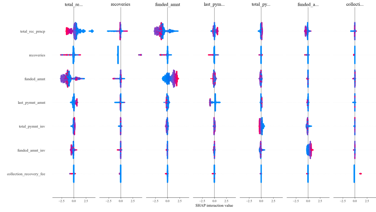
Figure 1. class1 Interaction diagram

3.5.2. SHAP diagram

The SHAP diagram shows the decomposition of the predicted value of a single sample, showing how each feature pushes the predicted value up or down. Through the diagram, we can clearly see the positive and negative effects of each feature on the model output, and the result of their combined action.

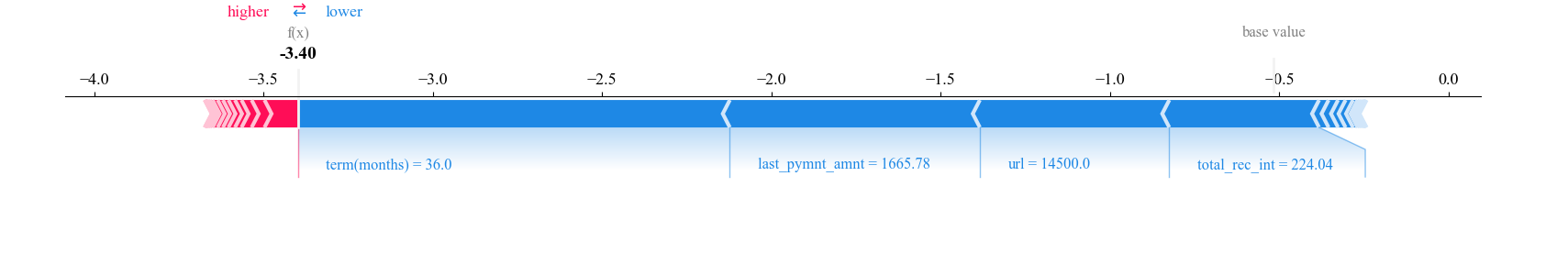
Figure 2. class2 diagram

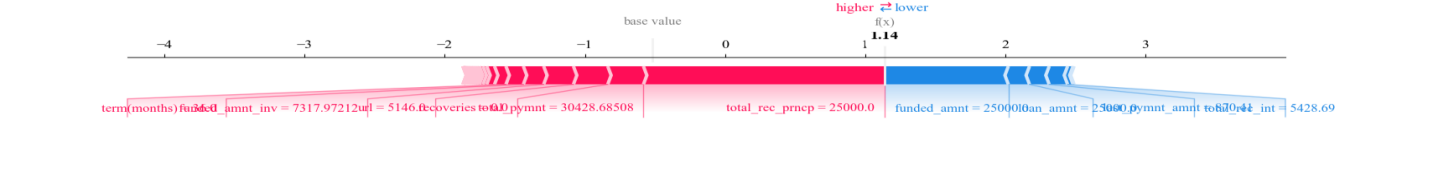
Figure 3. class3 attempt

3.5.3. SHAP heat map

The SHAP heat map shows the feature contribution of multiple samples, where the color gradient indicates the size of the SHAP value. From this map, it is possible to identify which features have consistent effects across samples and how these effects change across samples.

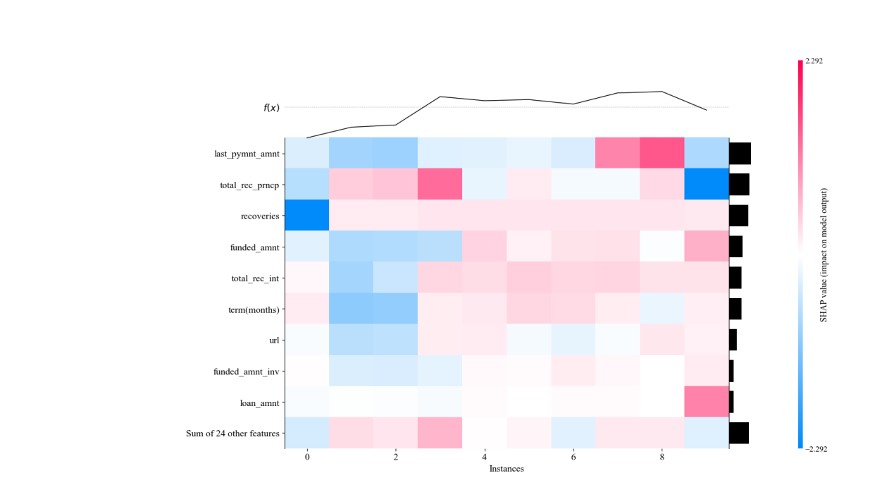
Figure 4. class3 heat map

3.5.4. General SHAP map

The SHAP general diagram provides an overview of the importance of all the features in the model. Each point in the plot represents the SHAP value of a sample, and the color indicates the size of that feature value. By summarizing the graph, it is possible to identify the features that are most important to the model's predictions, and the direction in which these features influence on a global scale, which is critical to understanding the overall behavior of the model.

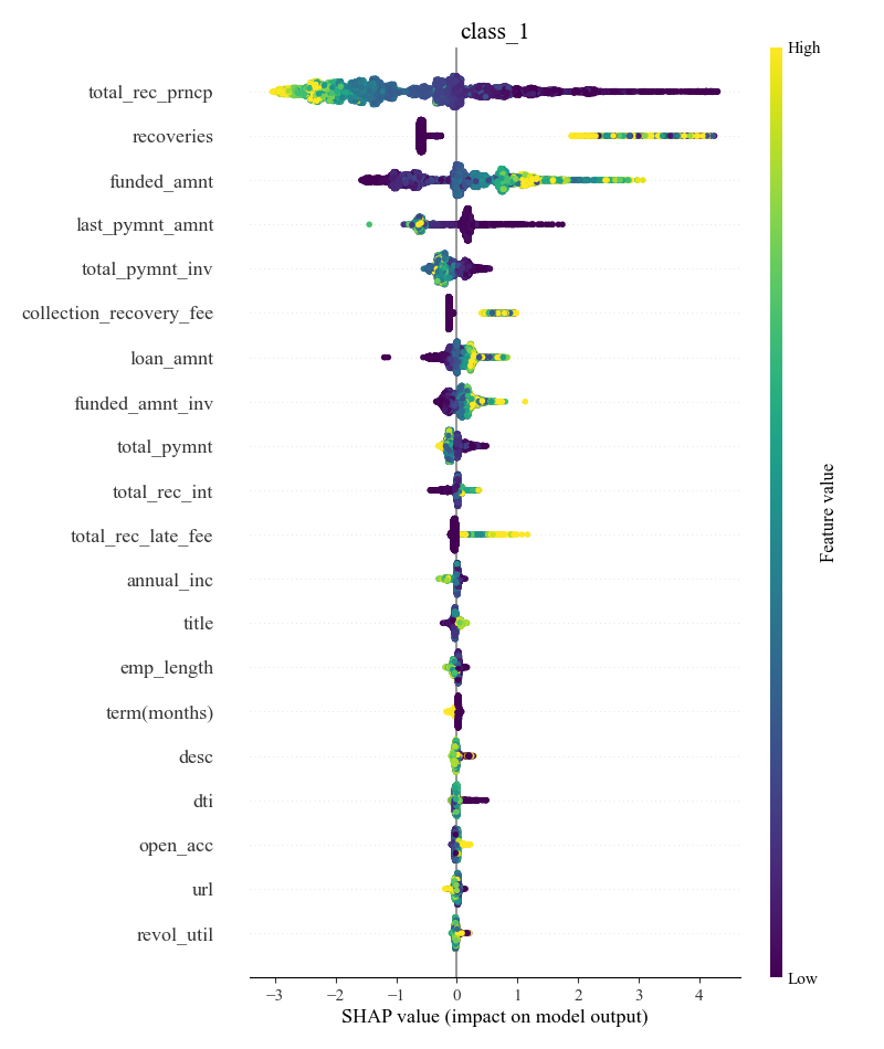
Figure 5. class1 General diagram

To gain a deeper understanding of the model's prediction mechanism, we calculated the contribution of each feature by using the feature importance measure inside the XGBoost model. According to the calculated results, we find that the feature "total_rec_pmcp" has the highest importance, followed by the feature "last_pymnt_amnt" and the feature "funded_amnt".

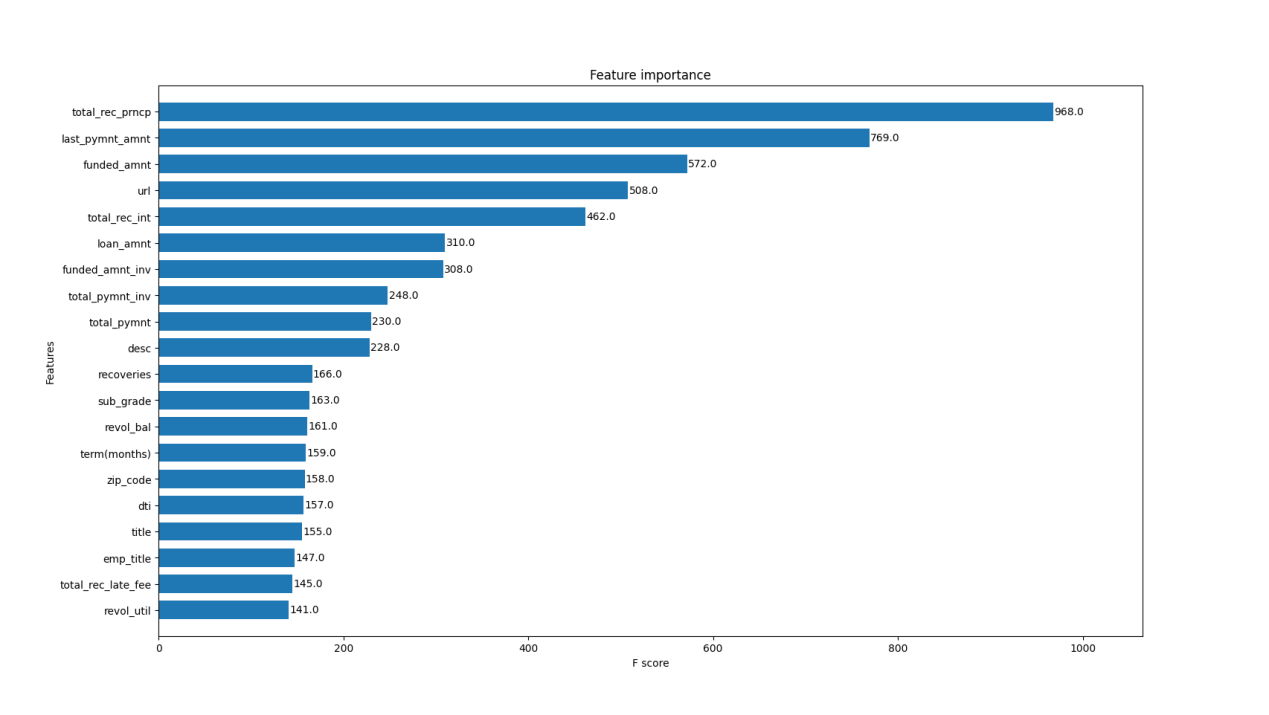
Figure 6. Prioritization of the original feature

We further verified these results by Permutation Importance, finding that the perturbation of the feature "total_rec_pmcp" significantly reduces the model performance, followed by the feature "funded_amnt" and the feature "recoveries", which are basically consistent with the results of SHAP.

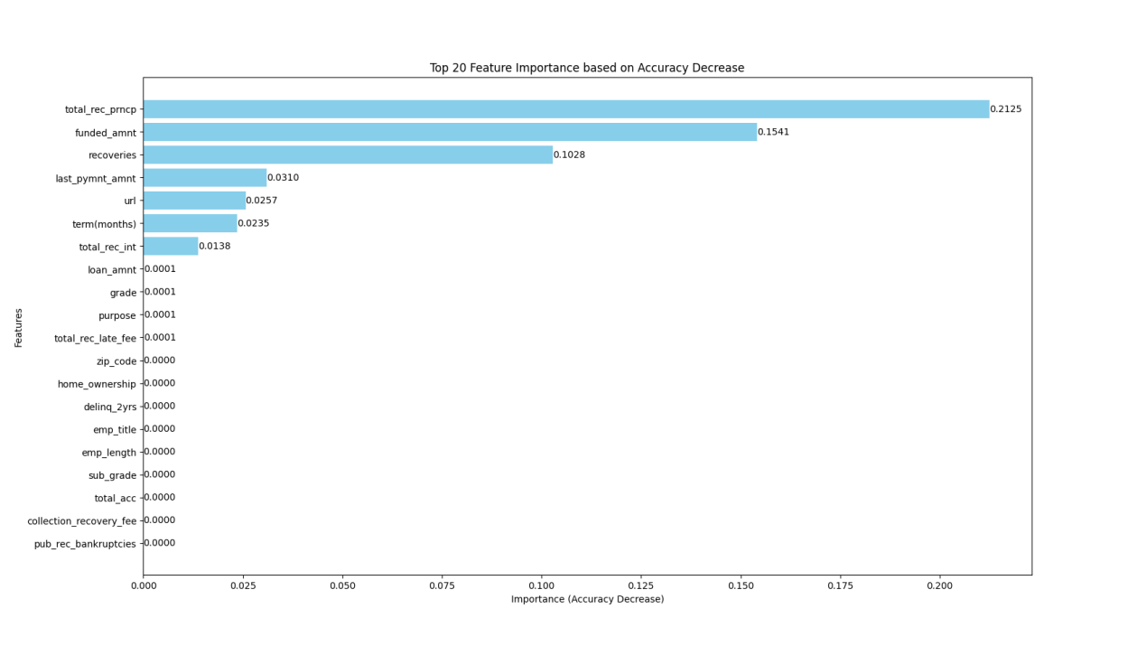
Figure 7. Feature importance ranking after shuffling

'total_rec_prncp' stands for principal paid and refers to the amount of principal paid back by the borrower over the life of the loan. The more the principal has been paid, the less the remaining loan. It usually means that the borrower has strong repayment willingness and repayment ability, can repay the principal on time or in advance, and the possibility of loan default is low.

'funded_amnt' stands for financing amount, which refers to the total amount of loans the borrower applies for and receives. The larger the financing amount, the greater the pressure on the borrower to repay. High loan requires the borrower to have a higher income and good financial status to repay on time, so the risk of the loan is also higher.

'recoveries' represent recoveries after a borrower defaults, and refer to the amount of money that the lender is able to recover after the borrower defaults, including possible liquidated damages. The higher the recovery amount after default, the more the lender will be able to reduce losses if the borrower defaults, reducing the risk of the overall loan portfolio. For borrowers, higher liquidated damages can act as a deterrent to avoid default as much as possible.

Based on the above practical analysis, these characteristics that have a greater impact on the result can indeed reflect the borrower's repayment ability, loan risk and possible loss after default, so they have an important impact on loan prediction, and also show the correctness and advanced nature of the two interpretation and analysis methods.

4. Conclusion

In this study, the open data set from Lending Club is used as the experimental data set. Firstly, the data is cleaned, the useless features are deleted, and the non-digital variables are digitized. Then, through comparative analysis of multiple machine learning algorithms (including SVM, XGBoost, Random Forest, Bayesian and Decision Tree), we find that the accuracy, accuracy, recall and F1 scores of the XGBoost model are all around 0.9942. Which is higher than the other models, so we choose it as the subsequent benchmark model. In addition, through SHAP and replacement importance, we conduct a feature importance analysis. The results show that the two methods show that the principal paid by the borrower, the financing amount and the recovery amount after the borrower defaults are three important factors affecting the loan approval. The results show that the loan prediction model based on machine learning can significantly improve the accuracy of banks' decision making in the loan approval process and help financial institutions manage risks more effectively. However, this study also has some limitations, our model is mainly based on static data, and more dynamic features, such as real-time credit scores and market changes, can be considered in the future. Secondly, more diverse and larger data sets can be collected and analyzed to improve the generalization ability of the model.

References

[1]. Naseer S, Khalid S, Parveen S, et al. COVID-19 outbreak: Impact on global economy[J]. Frontiers in public health, 2023, 10: 1009393.
[2]. Rekunenko I, Zhuravka F, Nebaba N, et al. Assessment and forecasting of Ukraine’s financial security: Choice of alternatives[J]. 2023.
[3]. Dansana D, Patro S G K, Mishra B K, et al. Analyzing the impact of loan features on bank loan prediction using R andom F orest algorithm[J]. Engineering Reports, 2024, 6(2): e12707.
[4]. Rana M, Bhushan M. Machine learning and deep learning approach for medical image analysis: diagnosis to detection[J]. Multimedia Tools and Applications, 2023, 82(17): 26731-26769.
[5]. Lee D H, Chen K L, Liou K H, et al. Deep learning and control algorithms of direct perception for autonomous driving[J]. Applied Intelligence, 2021, 51(1): 237-247.
[6]. Sujatha C N, Gudipalli A, Pushyami B, et al. Loan prediction using machine learning and its deployement on web application[C]//2021 Innovations in Power and Advanced Computing Technologies (i-PACT). IEEE, 2021: 1-7.
[7]. West D. Neural network credit scoring models[J]. Computers & operations research, 2000, 27(11-12): 1131-1152.
[8]. Kumari K, Jayarathna H. Predicting Income and Feasible Loan Amount for a Household Unit (Expenditure Analysis of Badulla District, Sri Lanka)[J]. 2019.
[9]. Khilfah H N L, Faturohman T. Social media data to determine loan default predicting method in an Islamic online P2P lending[J]. Journal of Islamic Monetary Economics and Finance, 2020, 6(2): 243-274.
[10]. Manglani R, Bokhare A. Logistic regression model for loan prediction: A machine learning approach[C]//2021 Emerging Trends in Industry 4.0 (ETI 4.0). IEEE, 202:1-6.
[11]. Madaan M, Kumar A, Keshri C, et al. Loan default prediction using decision trees and random forest: A comparative study[C]//IOP conference series: materials science and engineering. IOP Publishing, 2021, 1022(1): 012042.
[12]. Zhu Q, Ding W, Xiang M, et al. Loan default prediction based on convolutional neural network and LightGBM[J]. International Journal of Data Warehousing and Mining (IJDWM), 2023, 19(1): 1-16.
[13]. Zhu M, Zhang Y, Gong Y, et al. Ensemble methodology: Innovations in credit default prediction using lightgbm, xgboost, and localensemble[J]. arXiv preprint arXiv:2402.17979, 2024.
[14]. Anh N T T, Hanh P T M, Le Thu V T. Default in the US peer-to-peer market with covid-19 pandemic update: An empirical analysis from lending club platform[J]. International Journal of Entrepreneurship, 2021, 25(7): 1-19.
[15]. Murimi L N, Siebert M, Salira G, et al. A Loan Application Management System for Efficient Loan Processing: A Case of Muhimbili SACCOS LTD[C]//International Conference on Technological Advancement in Embedded and Mobile Systems. Cham: Springer Nature Switzerland, 2022: 129-141.
[16]. Chakraborty S, Tomsett R, Raghavendra R, et al. Interpretability of deep learning models: A survey of results[C]//2017 IEEE smartworld, ubiquitous intelligence & computing, advanced & trusted computed, scalable computing & communications, cloud & big data computing, Internet of people and smart city innovation (smartworld/SCALCOM/UIC/ATC/CBDcom/IOP/SCI). IEEE, 2017: 1-6.
[17]. Garnica-Caparros M, Memmert D. Understanding gender differences in professional European football through machine learning interpretability and match actions data[J]. Scientific reports, 2021, 11(1): 10805.
[18]. Garreau D, Luxburg U. Explaining the explainer: A first theoretical analysis of LIME[C]//International conference on artificial intelligence and statistics. PMLR, 2020: 1287-1296.
[19]. Gramegna A, Giudici P. SHAP and LIME: an evaluation of discriminative power in credit risk[J]. Frontiers in Artificial Intelligence, 2021, 4: 752558.
[20]. Chen T, Guestrin C. Xgboost: A scalable tree boosting system[C]//Proceedings of the 22nd acm sigkdd international conference on knowledge discovery and data mining. 2016: 785-794.
[21]. Lundberg S M, Lee S I. A unified approach to interpreting model predictions[J]. Advances in neural information processing systems, 2017, 30.
[22]. Jabeur S B, Mefteh-Wali S, Viviani J L. Forecasting gold price with the XGBoost algorithm and SHAP interaction values[J]. Annals of Operations Research, 2024, 334(1): 679-699.
Cite this article
Cui,B. (2024). Loan Forecasting Based on Machine Learning and Variable Correlation Analysis. Applied and Computational Engineering,107,127-138.
Data availability
The datasets used and/or analyzed during the current study will be available from the authors upon reasonable request.
Disclaimer/Publisher's Note
The statements, opinions and data contained in all publications are solely those of the individual author(s) and contributor(s) and not of EWA Publishing and/or the editor(s). EWA Publishing and/or the editor(s) disclaim responsibility for any injury to people or property resulting from any ideas, methods, instructions or products referred to in the content.
About volume
Volume title: Proceedings of the 2nd International Conference on Machine Learning and Automation
© 2024 by the author(s). Licensee EWA Publishing, Oxford, UK. This article is an open access article distributed under the terms and
conditions of the Creative Commons Attribution (CC BY) license. Authors who
publish this series agree to the following terms:
1. Authors retain copyright and grant the series right of first publication with the work simultaneously licensed under a Creative Commons
Attribution License that allows others to share the work with an acknowledgment of the work's authorship and initial publication in this
series.
2. Authors are able to enter into separate, additional contractual arrangements for the non-exclusive distribution of the series's published
version of the work (e.g., post it to an institutional repository or publish it in a book), with an acknowledgment of its initial
publication in this series.
3. Authors are permitted and encouraged to post their work online (e.g., in institutional repositories or on their website) prior to and
during the submission process, as it can lead to productive exchanges, as well as earlier and greater citation of published work (See
Open access policy for details).