1. Introduction

Tennis, as a globally popular sport, has always attracted the attention of audiences, athletes, and researchers due to its complexity and unpredictability in competition. In this competitive sport, the rhythm and dynamics of the competition are often unexpected, and this phenomenon is often attributed to a concept called "momentum" [1]. The definition of momentum in the dictionary is "the force or force obtained through motion or a series of events." However, although this concept is widely accepted in sports competitions, its specific meaning, mechanism of generation, and how to quantify it are still unresolved issues.

The Wimbledon Open, as one of the four Grand Slam tournaments, is renowned for its unique rules and strict discipline of play [2]. In Wimbledon, players need to score through various methods, including serving, receiving, scoring in front of the net, and long shots from the baseline. At the same time, the competition state of the contestants will also change with the progress of the competition, including the consumption of physical energy, changes in psychological pressure, fluctuations in technical status, etc. These factors will all affect the dynamics and results of the competition, which is what we call momentum.

The Guardian wrote in a report on changes in the state of tennis players: "In tennis matches, a player's state of change often determines the outcome more than their skills and tactics. This is what we often call 'momentum', which is intangible but can determine the direction of the game." This viewpoint reveals the importance of 'momentum' in tennis matches and provides valuable insights for our research [3,4]. To address the enigmatic nature of momentum, we propose a multifaceted approach:

We will develop a model using the fuzzy comprehensive evaluation method to identify which player is performing better at any given time during a match, providing a visual representation of the game's progression. To counter skepticism about the role of momentum, we will employ the ARIMA model to analyze time series data, demonstrating the influence of momentum on match outcomes. We aim to predict momentum fluctuations using a quantification model, identifying the most relevant factors and suggesting strategies for upcoming matches.

2. Models

We have developed a model using the fuzzy comprehensive evaluation method to determine which tennis player performs better at specific game moments and visualize the game's progress. To address skepticism about the randomness of player success, we applied the ARIMA model to analyze time series data, capturing dynamic performance changes. Additionally, we used momentum quantification models to predict game fluctuations based on data from past matches.

2.1. Fuzzy comprehensive evaluation model

2.1.1. Data collection and preprocessing We first split the entire game into sets and games, and then delete the previous sets and games information to simplify the table. Next, we will convert the score into forms such as 0, 1, 2, etc. according to the rules of tennis matches, which makes it easier for us to calculate the score difference. There are two players in a game, and we only select one player for analysis. Considering the different factors considered in the serving and receiving situations, it is necessary to analyze the data of the serving and receiving situations separately.different speed limits.

2.1.2. Determination of evaluation indicators

• Service Game

We set the evaluation criteria for serving as scoring efficiency, serving quality (ball speed, ACE times, double serve errors), and non forced errors. We use the following equation to calculate the scoring efficiency:

\( Scoring efficiency=\frac{The number of rounds in this round}{The score in this round} \) (1)

The reason for selecting the number of rounds as a variable is that not all times of a game are played, such as when there is time to prepare for serving or when a challenge is requested. The time difference given in the second column of the table cannot be used for calculation. Only the number of rounds can reflect the true effective time of the game. This equation is equivalent to "frequency", which means that obtaining one point requires several rounds. When a player is in his serve, he will gain an additional advantage, so it is necessary to measure the player's ability to grasp the advantage, that is, the quality of his serve. So we created a simple formula to measure an athlete's serving level:

\( ServeQuality=α*ServeSpeed±β*ACEs∓ \) γ \( * \) DoubleFaults (2)

Among them \( α,β,γ \) are weight parameters that can be set based on your understanding of the importance of each factor, or can be learned through data training.

This formula assumes that the speed of the ball and the number of ACEs are directly proportional to the quality of the serve (i.e., the higher these values, the better the quality of the serve), while the number of double serve errors is inversely proportional to the quality of the serve (i.e., the higher these values, the worse the quality of the serve). The weight parameter determines the degree to which each factor affects the quality of serve. For example, if we believe that ACE counts are more important than ball speed, then β It should be better than \( α \) Big.

When a player voluntarily makes a mistake when the opponent does not play a threatening ball, it indicates that the player may have a fluctuating mentality or insufficient concentration, which affects the overall performance score.

• Receiving game

We set the evaluation criteria for receiving and serving games as scoring efficiency, return quality, and number of non forced errors. The evaluation methods of the above three criteria are similar to those of serving games.

2.1.3. The establishment of a fuzzy comprehensive evaluation model Firstly, we need to determine the series and basic framework.The basic principle of determining series is to follow the correlation of various evaluation indicators. If some indicators have strong correlation, we can consider dividing these indicators into the same level first. From this, we can conclude the basic framework of the model in Figure 1 [3].

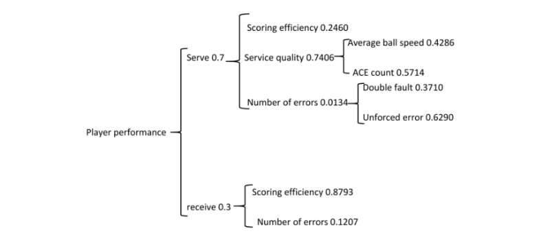
Figure 1. The basic framework of the model [3]

Next, we will determine the weights using the entropy weight method, with the following steps:

①Standardization: The purpose of standardization is to eliminate the influence of dimensionality between various indicators.

②Normalization: Evaluation data can be divided into large, small, intermediate, and interval types. The special type that this question may involve is small. For small data, we should normalize it to ensure consistency in the direction of the indicators.

③In order to better reflect the level of a certain data item in the overall data, we convert each data item into a "score". Because the characteristic of some data is that the numerical distribution is relatively concentrated, and after standardization, it tends to a narrow range. If such data also has the characteristic of small numerical differences reflecting large differences, its level needs to be measured through "scores".

④Obtain probability matrix.

⑤Calculate information entropy and information utility values [4]

⑥Calculate entropy weight [5]

Next, we will construct a comprehensive evaluation matrix and write a weight matrix. The specific ai value has been determined by the entropy weight method.

A=[α₁, α₂, ......,α_n] (3)

Then write a fuzzy judgment matrix. The fuzzy judgment matrix is composed of m indicators and m * n membership elements of n comments, where n is taken as 3 and the comment set is {excellent, good, poor}.

\( (\begin{matrix}{r_{11}} & ⋯ & {r_{1m}} \\ ⋮ & ⋱ & ⋮ \\ {r_{n1}} & ⋯ & {r_{nm}} \\ \end{matrix}) \) (4)

The method for determining the membership degree r:

Construct membership functions for each evaluation indicator regarding the comment set, using the membership function of ball speed as an example:

Firstly, we perform cluster analysis on a large amount of data to obtain three cluster centers, divide the ball velocity into four intervals, and determine the segmented membership function (for ease of operation, the critical value of the segmented function is taken as the approximate value of the cluster center)

Poor membership function:

\( Y=\begin{cases} \begin{array}{c} 1 x \lt =95 \\ -0.067x+7.33 95 \lt x \lt 110 \\ 0 x \gt =110 \end{array} \end{cases} \) (5)

Good membership function:

\( Y=\begin{cases} \begin{array}{c} 0 x \lt =95 \\ 0.067x+6.33 95 \lt x \lt =110 \\ -0.1x+12 110 \lt x \lt =120 \\ 1 x \gt 120 \end{array} \end{cases} \) (6)

Excellent membership function:

\( Y=\begin{cases} \begin{array}{c} 0 x \lt =110 \\ 0.1x+11 110 \lt x \lt 120 \\ 1 x \gt =120 \end{array} \end{cases} \) (7)

From this, we can obtain a comprehensive evaluation matrix B for a certain level: B=A * R, where matrix B is a matrix that can be considered as a row vector.Then, further obtain the comprehensive judgment matrix R of the upper level, and combine the row vectors of the lower level evaluation into a matrix, which will result in a matrix with the same number of rows as the upper level evaluation indicators

\( {R={B_{i}}∈R^{Kx1}} \) (8)

Repeat the above process twice to obtain the final comprehensive evaluation matrix.

2.2. ARIMA model

2.2.1. Understanding momentum Momentum is a constantly changing value that is related to the performance of players in various aspects during the competition. If there is no influence of momentum in the competition, the inherent strength of the two individuals will become the only influencing factor. On the contrary, if there is momentum, whether a player can score the next point will depend to some extent on their previous performance. The current performance will form a time series equation with the previous performance, and the previous performance is represented by several lag terms on the right side of the equal sign.

\( X_{t+1}^{*} \) =α₁x_t \( + \) α₁(1-α₁)x_t-1 \( + \) α₁(1-α₁)²x_t-2+......+α₁(1-α₁)^t-1x₁+(1-α₁)^tl₀ (9)

l₀ =X₁^* (10)

From this equation, we can see that the closer the data is to the current period, the greater the weight. This is in line with our starting point of verifying whether the recent performance in sports competitions has an impact on the current performance and the extent of the impact.

2.2.2. Verify autocorrelation The autocorrelation coefficient is the hub between predicted and observed values, and is also the key to verifying autocorrelation. According to the knowledge of probability theory, the definition formula of autocorrelation coefficient is [2]:

^ρ_s= \( \frac{cov({x_{t}},{x_{t-s}})}{[{var({x_{t}})^{0.5}}*{var({x_{t-s}})^{0.5}}]} \) (11)

The above equation only applies to certain special conditions, and a simple form of autocorrelation coefficient can be obtained. The true autocorrelation coefficient needs to be calculated based on the specific values of the observed values. The formula is as follows:

\( {γ_{s}}=ρ_{s}^{*}=\frac{\sum _{t=s+1}^{ρ}({x_{t}}-{x_{average}})({x_{t-s}}-{x_{average}})}{\sum _{t=1}^{ρ}{({x_{t}}-{x_{average}})^{2}}} \) (12)

We used Python to draw an image of the autocorrelation coefficient (on the right is the image of the partial autocorrelation coefficient, obtained together (Figure 2))

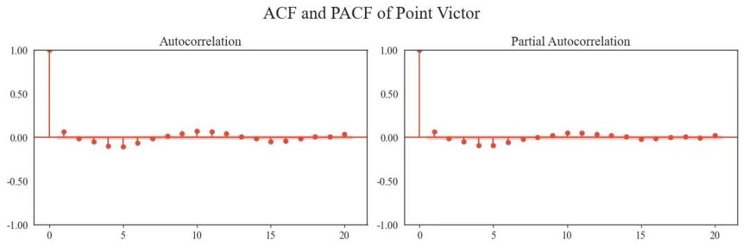
Figure 2. Acf and Pacf of point victor (Photo/Picture credit : Original)

From the figure 2, it can be seen that there is a clear correlation between whether one can obtain this point and many previous performances. Therefore, it can be concluded that there is a momentum effect in the game, and the coach's statement is incorrect. The ARIMA model, with its three main parameters (autoregressive term, number of differences, and moving average term), offers both simplicity in understanding and interpretation. It is flexible enough to handle various types of time series data, whether stationary or non-stationary, trending or not. Moreover, ARIMA models have demonstrated strong predictive abilities, particularly for data exhibiting clear trends.

2.3. Momentum quantification model

Momentum, as an abstract term, reflects an athlete's momentum during a game. Based on their recent scoring performance, we can determine the strength of their momentum. If other influences are not considered, the scoring situation of two players in the past few goals should be split in half, and the deviation between the actual scoring probability and the theoretical value reflects the strength of the player's momentum. We use a binomial distribution to calculate the probability of the player winning a certain number of points and set a "window" to determine the scope of discussion.

X~B(n,p) (13)

Window size is len (odd).The probability of this event is calculated based on the window centered on i, assuming that the player has won n times:

\( P(X=n)=C_{len}^{n}{(\frac{1}{2})^{n}}{(\frac{1}{2})^{len-n}} \) (14)

From this expression, it can be seen that the probability of winning n times depends entirely on the size of the previous Cn len. According to the discrete value distribution map of Cn len, the more times one wins or loses, the smaller the probability, and the maximum probability approaches 1/2.

① If the number of wins is less than len/2, it indicates that the momentum is biased towards the opponent, represented by a negative number

Momentum=- (0.5-P (x=n)) (15)

② If the number of wins is greater than len/2, it indicates that the momentum is biased towards that player, represented by a positive number

Momentum=0.5-P (x=n) (16)

③In order to distinguish the differences between numerical values more clearly, we multiply this value by 2 and enlarge it to between (-1,1)

④ In order to make the momentum quantification values we defined more universal, we took different window sizes, 31, 15, 7, and 3 respectively, calculated their momentum values, and calculated the weighted average of these values (the weight is the size of the current window)

Obtain the final expression for momentum magnitude:

\( M=\frac{\sum len*f(len)}{\sum len} \) (17)

2.4. Predicting match fluctuations - LSTM

LSTM is an advanced version of traditional recurrent neural networks [6]. The disadvantage of recurrent neural networks [7,8] is that they are prone to the problem of vanishing gradients during backpropagation, and gradients are a key factor used to update the weights of neural networks. If the gradient is too small, then it makes little contribution to the learning of the network, resulting in ineffective learning of layers with very small gradient updates in recurrent neural networks, which are usually earlier layers. Therefore, recurrent neural networks are prone to forgetting information from longer time series.

LSTM can effectively solve short-term memory problems through its cellular state. It acts like an information highway, continuously transmitting early information throughout the entire sequence, helping to weaken the limitations of short-term memory. In its flow path, information will go through various "gates" for filtering or deletion from the cell state, and the "gates" will learn to filter and forget information during the training process.

3. Experimental result

3.1. Dataset and evaluation metrics.

Firstly, we checked the integrity and accuracy of the data. We found that match number 2023-wimbledon-1310 lacks information related to serving. In the process of processing data, we found significant differences between some data and most other game data. For these outliers, we will decide whether to retain, modify, or delete them according to the needs of the model. After data cleaning, there will be 7114 data available for use. Based on the actual needs of the problem, we will use the processed data to create new features for standardization (Figure 3 and Figure 4).

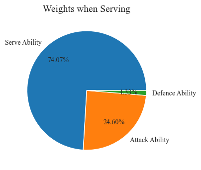
Figure 3. The proportion of players' serving and non serving abilities (Photo/Picture credit : Original)

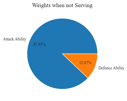
Figure 4. The establishment of a fuzzy comprehensive evaluation model (Photo/Picture credit : Original)

After calculating the score, we visualized the score point difference means who has the advantage of small game points (Figure 5).

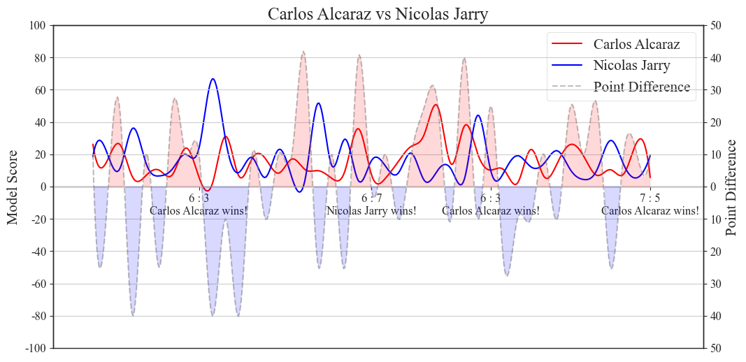
Figure 5. Scoring situation of Carlos Alcaraz and Nicolas Jarry in tennis matches. (Photo/Picture credit : Original)

Through this chart, we can clearly see the scoring situation of Carlos Alcaraz and Nicolas Jarry in tennis matches. The red line represents Carlos Alcaraz's score, the blue line represents Nicolas Jarry's score, and the gray line represents the difference in scores between the two. In addition, the chart also displays the scores of the players in the captured game window, helping us better understand the progress of the game.

Through the figure 5, we can clearly observe the relationship between Carlos and Nicolas' comprehensive score determination and the outcome of the next game, indicating that our model accurately provides the changes in the momentum of players under different score situations

Quantitative analysis uses mathematical models to objectively and accurately analyze the competition. It dynamically displays changes over time, allowing for a clear visualization of player performance shifts during the game, thus aiding in understanding the dynamic process and momentum changes. This method considers multiple factors such as ball speed, ACE counts, and double serve errors, providing a comprehensive evaluation of a player's performance. It is also highly flexible, as weight parameters can be adjusted according to specific situations, enabling the model to prioritize certain aspects like the number of ACEs if deemed more important than others.

3.2. Analysis and prediction based on LSTM model

3.2.1. Plot the game momentum fluctuations We selected the match data of two players, Carlos Alcaraz and Novak Djokovic, from the data file for prediction. First, we drew the momentum change chart with Carlos Alcaraz as the research object. Therefore, the part with negative momentum below the center axis represents the momentum dominance of Novak Djokovic (Figure 6).

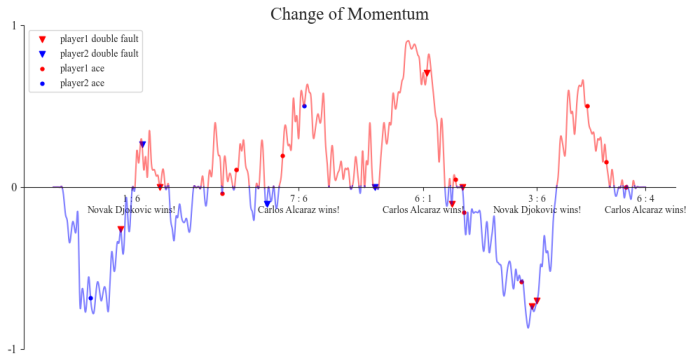
Figure 6. The momentum change chart with Carlos Alcaraz as the research object (Photo/Picture credit : Original)

Compared with the original data, we marked the factors that may affect the momentum transition in the figure, including double faults and ACE. After the completion of the marking, we found that if the player can serve ACE, the momentum will be significantly increased, while if the player has double faults, the momentum will be significantly decreased. Figure 7 is a rendering of our prediction

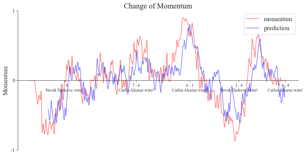
Figure 7. Rendering of our prediction (Photo/Picture credit : Original)

The window length of this prediction image is 31:15:7:3. Who served the first 24 balls, whether there was an ace, who scored, whether there was a double fault, whether there was an unforced error, predict the current momentum

The average absolute error and mean square error of the LSTM model on the test set are 0.0883 and 0.0095, respectively. These indicators indicate that the model has high prediction accuracy and stability, and can effectively capture the dynamic changes of the game. Overall, the LSTM model performs well in predicting changes in kinetic energy during tennis matches and has good application prospects.

3.2.2. Factors associated with volatility By analyzing the momentum changes at this time and the next time, we can determine the degree of influence of these factors.

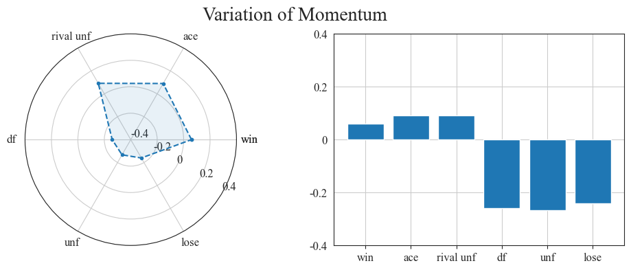
Figure 8. Variation of momentum (Photo/Picture credit : Original)

In the statistical chart of dynamic changes and competitive strategies (Figure 8), Ace (direct serve score) is a positive attribute, indicating the advantage of the serving party; Rival unf is also a positive attribute, reflecting our ability to apply pressure; Df (our double mistake failure) and unforced error Unf are negative attributes that reflect technical errors and game stability, respectively.

3.2.3. Generalization of the model In order to evaluate the generalization ability of the model, we selected a table tennis match and a volleyball match for prediction, and the prediction results were as figure 9:

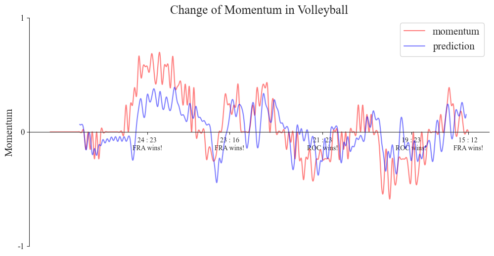
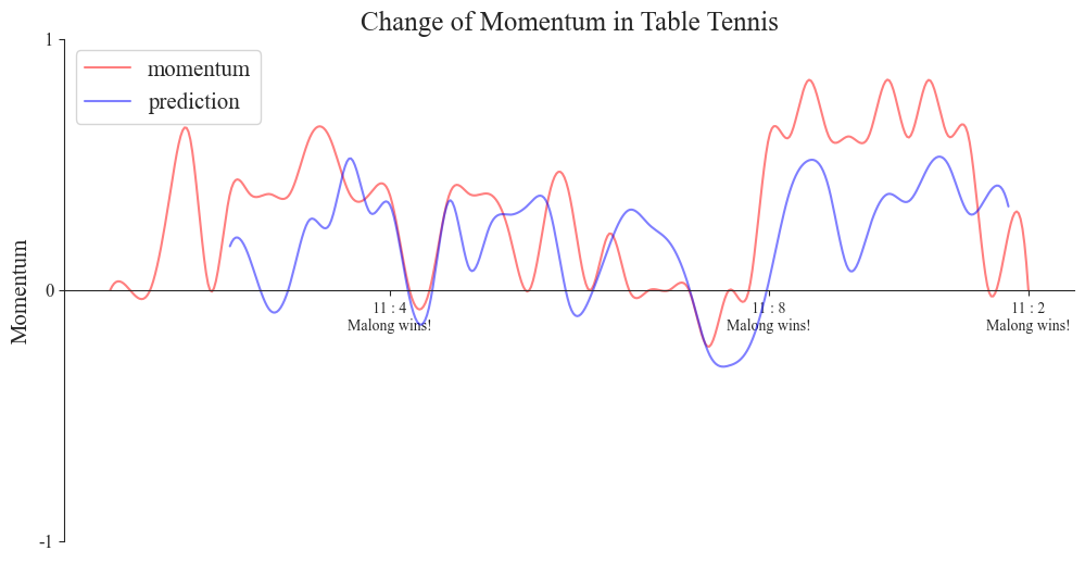
Figure 9. Prediction results (Photo/Picture credit : Original)

It can be seen that the prediction effect of the model is better in table tennis, but not so much in volleyball. There are certain differences between these two kinds of games and tennis, especially volleyball is a team sport, and more team factors need to be considered. Overall consideration, the factors to be included are: the double strength gap is too large (can introduce the amount of correction), the change of players in the game, tactical pause and so on.

The accuracy of the model is obtained by calculating MSE and MAE.

Table 1. The result of MAE and MSE

Based on the provided data, we can draw the following conclusions (Table 1): The MAE of the first experiment was 0.1162, and the MAE of the second experiment was 0.0818. This indicates that the average absolute error of the prediction results has decreased when testing the model on table tennis. The MSE of the first experiment is 0.0193, and the MSE of the second experiment is 0.0099. This indicates that the mean square error of the prediction results has been reduced when testing the model on table tennis. In summary, by using the LSTM model to test the generalization ability of the tennis model on table tennis, we found that the average absolute error and mean square error of the prediction results were reduced, indicating that the model performs well on table tennis. The LSTM model, a powerful tool for time series analysis, captures long-term dependencies in data, enhancing our understanding and prediction of momentum changes in competitions. Our method, analyzing multiple game elements like point difference, consecutive scoring, mistakes, ACEs, and service breaks, offers a comprehensive approach to accurately predict these shifts. By annotating momentum fluctuations in the original data graph, we enable a more intuitive grasp and precise analysis of the reasons behind these changes.

4. Conclusion

Alcaraz's performance was characterized by a remarkable vitality that set him apart, as he skillfully capitalized on scoring opportunities and break points to widen his lead. To delve deeper into the concept of momentum, we employed a rigorous quantitative approach, measuring it by calculating the deviation between the actual probabilities of scoring occurrences during play and those predicted by a theoretical binomial distribution. This method allowed us to quantify the extent to which a player's scoring patterns deviated from randomness, thereby capturing the essence of momentum. For predicting changes in momentum, we turned to advanced machine learning techniques, specifically leveraging LSTM networks. These recurrent neural networks are adept at handling sequences of data and overcoming the limitations of short-term memory, making them ideally suited for analyzing the temporal dynamics of momentum in tennis matches. By embedding various contextual cues such as score differentials, streaks of consecutive points, unforced errors, aces, and successful breakpoints into our model, we were able to gain insights into the factors driving momentum shifts. To assess the generalizability of our findings, we extended our analysis to other racket sports, conducting predictive comparisons using data from professional table tennis and volleyball matches. Despite inherent differences in the rules and gameplay of these sports, our model consistently highlighted the pervasive influence of momentum, albeit with some nuances due to variations in competitive structures.

Conclusively, armed with the insights gleaned from the comprehensive study, this work compiled a succinct yet informative memorandum for coaches. This document encapsulates our key findings and offers strategic recommendations aimed at helping coaches devise preemptive strategies or timely interventions during matches.

References

[1]. Carter Jr, W. H., & Crews, S. L. (1974). An analysis of the game of tennis. The American Statistician, 28(4), 130-134.
[2]. McLeod, A. I., & Li, W. K. (1983). Diagnostic checking ARMA time series models using squared‐residual autocorrelations. Journal of time series analysis, 4(4), 269-273.
[3]. Feng, S., & Xu, L. D. (1999). Decision support for fuzzy comprehensive evaluation of urban development. Fuzzy Sets and Systems, 105(1), 1-12.
[4]. Zhu, Y., Tian, D., & Yan, F. (2020). Effectiveness of entropy weight method in decision-making. Mathematical Problems in Engineering, 2020, 1-5.
[5]. Liang, J., Shi, Z., Li, D., & Wierman, M. J. (2006). Information entropy, rough entropy and knowledge granulation in incomplete information systems. International Journal of general systems, 35(6), 641-654.
[6]. Staudemeyer, R. C., & Morris, E. R. (2019). Understanding LSTM--a tutorial into long short-term memory recurrent neural networks. arv preprint arv:1909.09586.
[7]. Li, S., Li, W., Cook, C., Zhu, C., & Gao, Y. (2018). Independently recurrent neural network (indrnn): Building a longer and deeper rnn. In Proceedings of the IEEE conference on computer vision and pattern recognition (pp. 5457-5466).
[8]. Gupta, D. L., Malviya, A. K., & Singh, S. (2012). Performance analysis of classification tree learning algorithms. International Journal of Computer Applications, 55(6).
Cite this article
He,X. (2024). Attempt to Quantify Momentum in Sports Competitions. Applied and Computational Engineering,105,131-142.
Data availability
The datasets used and/or analyzed during the current study will be available from the authors upon reasonable request.
Disclaimer/Publisher's Note
The statements, opinions and data contained in all publications are solely those of the individual author(s) and contributor(s) and not of EWA Publishing and/or the editor(s). EWA Publishing and/or the editor(s) disclaim responsibility for any injury to people or property resulting from any ideas, methods, instructions or products referred to in the content.
About volume
Volume title: Proceedings of CONF-MLA 2024 Workshop: Neural Computing and Applications
© 2024 by the author(s). Licensee EWA Publishing, Oxford, UK. This article is an open access article distributed under the terms and
conditions of the Creative Commons Attribution (CC BY) license. Authors who
publish this series agree to the following terms:
1. Authors retain copyright and grant the series right of first publication with the work simultaneously licensed under a Creative Commons
Attribution License that allows others to share the work with an acknowledgment of the work's authorship and initial publication in this
series.
2. Authors are able to enter into separate, additional contractual arrangements for the non-exclusive distribution of the series's published
version of the work (e.g., post it to an institutional repository or publish it in a book), with an acknowledgment of its initial
publication in this series.
3. Authors are permitted and encouraged to post their work online (e.g., in institutional repositories or on their website) prior to and
during the submission process, as it can lead to productive exchanges, as well as earlier and greater citation of published work (See
Open access policy for details).