1. Introduction

Traditional neural networks, a foundational type of feedforward architecture, are inspired by biological neuron structures and consist of input, hidden, and output layers. Data flows through these layers sequentially, with neurons activated by weights and nonlinear activation functions. Training methods like Backpropagation (BP) effectively reduce error by minimizing the loss function, making these networks effective in tasks involving pattern recognition [1-2]. However, traditional neural networks process each input independently, making them inadequate for tasks involving sequential data where each data point depends on previous ones [3-4]. This limitation, especially prominent with increasing data volumes and demand for temporal knowledge extraction, restricts their effectiveness in applications like stock prediction [5].

Recurrent Neural Networks (RNNs) address this limitation by introducing temporal dependencies, allowing data connections across time steps. Unlike traditional models, RNNs retain information from previous steps within a looped architecture, enabling the network to process sequence data, such as stock price prediction, where past values affect current ones. This temporal connection allows RNNs to model more complex relationships; however, RNNs struggle with long-term dependencies due to gradient vanishing and explosion, issues that arise from the repeated use of weights over time [4]. These problems fundamentally limit the RNN’s ability to retain information from distant past steps, making it challenging to capture long-range dependencies [1-2]. To overcome these issues, Long Short-Term Memory (LSTM) networks were developed. LSTMs introduce a memory cell structure controlled by three gates—Input, Forget, and Output—that regulate information flow, selectively retaining or discarding information as needed. This gated mechanism mitigates gradient issues, making LSTM effective in handling long sequences while reducing the risks of overfitting [6-8]. LSTM’s architecture allows it to capture nonlinear and complex temporal patterns, making it particularly suited for stock prediction tasks where current data points are strongly influenced by historical trends and investor behavior.

This paper examines the evolution from traditional neural networks to RNN-based models, exploring their structures, benefits, and applications. After reviewing the basic architectures of RNNs and the advanced mechanisms of LSTM and Gated Recurrent Units (GRU), a detailed comparison is provided, highlighting each model’s capabilities and advantages in sequence data processing. Finally, an LSTM-based stock prediction system is constructed to illustrate how RNNs can effectively model time-dependent financial data. This study demonstrates how leveraging LSTM’s structure enhances forecasting accuracy in stock markets, where modeling temporal dependencies is essential.

2. Literature Review

2.1. Recurrent Neural Network

Even the traditional neural network has a strong learning and fitting ability to solve practical problems, but when faced with a sequence of data, text prediction, speech analysis, and so on, it can not complete the task well. Therefore, computer scientists create more advanced feedforward neural networks-Recurrent Neural Networks[1,6,9]. Unlike traditional neural networks, recurrent neural networks set up the concept of time in their internal parts, connecting the structure of cycles formed by edges across adjacent time steps. These cycles are connected to themselves at different time steps. At time t, the node of the loop receives the current input \( {x^{t}} \) , combines the input of the previously hidden state \( {h^{t-1}} \) , outputs the sum value \( {y^{t}}, \) and updates the hidden state used in the next step under the condition of the currently hidden state \( {h^{t}} \) , shown in Figure 1.

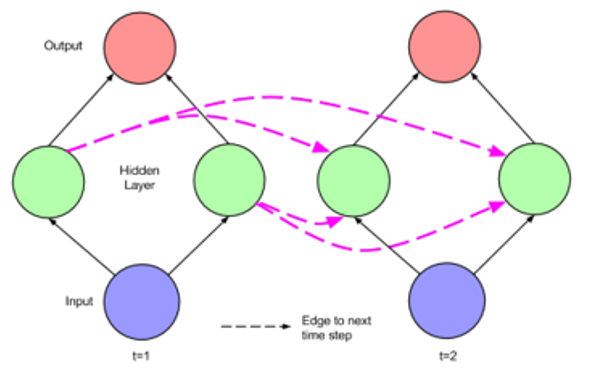
Figure 1. Simple Recurrent Network Unfolded Across Time Step.

The parameters here are calculated by:

\( {h^{(t)}}=σ({W^{hx}}{x^{(t)}}+{W^{hh}}{h^{(t-1)}}+{b_{h}}) \) (1)

\( {\hat{y}^{(t)}}=softmax({W^{yh}}{h^{(t)}}+{b_{y}}) \) (2)

Where \( {W^{hx}} \) represents the weights between the Input layer and the Hidden layer and \( { W^{hh}} \) represents the weights between the Hidden layer and itself at adjacent time steps. \( {b_{h}} \) and \( {b_{y}} \) are bias. This algorithm makes the unfolded network can be trained in different time steps with the BP algorithm which is called backpropagation through time (BPTT) [10-11].

2.2. Long Short-Term Memory

RNN architectures are widely used because of their powerful ability to deal with sequenced data, but the functions of memory also bring problems such as gradient explosion, gradient vanishing, and the long-term dependence problem on memory, so computer scientists have made sorts of variants based on ordinary RNNs, such as the generation of LSTM relives the problems of the gradient explosion and vanishing problems and process the problems faster [6-8].

The standard RNN model operates slowly and is prone to gradient vanishing issues due to its non-selective memory retention of data. To address these challenges, Hochreiter and Schmidhuber developed the LSTM model in 1997, it enhances the traditional RNN by introducing a specialized hidden layer, where each standard node is replaced by a memory cell illustrated in Figure 2. This memory cell includes a self-connected recurrent weight, stabilizing gradients and effectively mitigating both gradient explosion and vanishing problems [6-7,11]. Utilizing this memory cell structure, LSTM incorporates input, forget, and output gates, which selectively retain relevant information while discarding unnecessary data. This gated mechanism allows LSTM to efficiently handle long-term dependencies in sequential data [9].

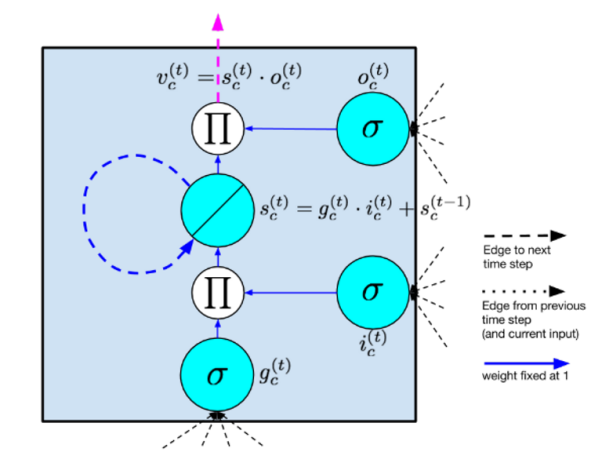
Figure 2. Long Short-Term Memory Structure

The parameters in Figure 2 are calculated in sequence by:

\( {g^{(t)}}=∅({W^{gx}}{x^{(t)}}+{W^{gh}}{h^{(t-1)}}+{b_{g}}) \) (3)

\( {g^{(t)}}=σ({W^{ix}}{x^{(t)}}+{W^{ih}}{h^{(t-1)}}+{b_{i}}) \) (4)

\( {f^{(t)}}=σ({W^{fx}}{x^{(t)}}+{W^{fh}}{h^{(t-1)}}+{b_{f}}) \) (5)

\( {o^{(t)}}=σ({W^{ox}}{x^{(t)}}+{W^{oh}}{h^{(t-1)}}+{b_{o}}) \) (6)

\( {s^{(t)}}={g^{(t)}}⊙{i^{(i)}}+{s^{(t-1)}} \) (7)

\( {h^{(t)}}=Ø({s^{(t)}}){⊙o^{(t)}} \) (8)

Where ⊙ represents the pointwise multiplication, \( {x^{(t)}} \) represents input layers, and \( {h^{(t)}} \) represents hidden layers.

2.3. Gated Recurrent Unit

GRU is a variant of LSTM which is relatively simpler and it combines the Forget gate and the Output gate into a new Update gate, which greatly reduces the training time shown in Figure 3.

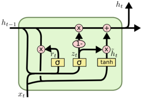
Figure 3: Gated Recurrent Unit Structure

Which can be calculated as:

\( {z_{t}}=σ({W_{z}}∙[{h_{t-1}},{x_{t}}]) \) (9)

\( {r_{t}}=σ({W_{r}}∙[{h_{t-1}},{x_{t}}]) \) (10)

\( {\widetilde{h}_{t}}=tanh(W∙[{r_{t*}}{h_{t-1}},{x_{t}}]) \) (11)

\( {h_{t}}=(1-{z_{t}})*{h_{t-1}}+{z_{t}}*{\widetilde{h}_{t}} \) (12)

In the face of relatively simple sequenced data that needs to be processed quickly, GRU can complete the task more efficiently than LSTM, and the accuracy is also guaranteed, which can better satisfy the demand of the tasks [7-8].

3. Methodology and Implementation

Stock trading data exhibits rhythmic patterns that can be effectively analyzed through numerical representation. Guided by statistical principles, such as the law of large numbers, stock behavior can be approximated and forecasted through machine learning models. In this research, various neural network architectures—including MLP (Multilayer Perceptron), RNN, GRU, and LSTM—were tested for stock price prediction. Due to BRNN's (Bidirectional RNN) need for entire data sequences to make specific predictions, it was not included in this comparison. The experiment utilized a dataset with 6,110 consecutive time points of a NASDAQ stock, from 1991 to 2016, containing features such as the date, previous closing price, opening price, maximum price, and daily increase, with the opening price of the next day as the target label. The dataset was divided into a 90% training set and a 10% test set to evaluate model performance.

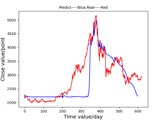
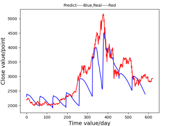
Figure 4. Prediction Graph of MLP Figure 5. Prediction Graph of RNN

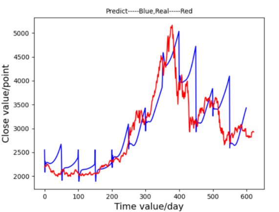
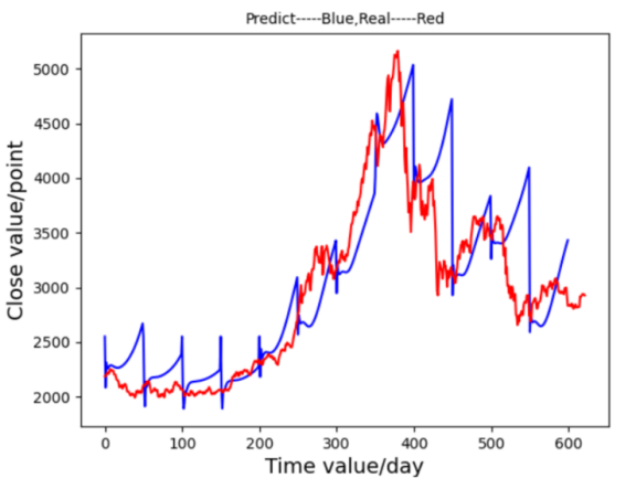
Figure 6. Prediction Graph of GRU Figure 7. Prediction Graph of LSTM

First, an MLP model was implemented with 10 input nodes, three hidden layers, and sigmoid activation functions. After 34 minutes of training, the MLP model produced a loss value of 89.73162, showing a limited fit to the stock trends, as observed in Figure 4. RNN was then employed, designed with two hidden layers and tanh activation. RNN achieved improved accuracy, with a loss of 3.87293 and a training time of approximately 22 minutes, as shown in Figure 5, capturing the overall trend more accurately despite some excessive volatility. The primary focus of this research, LSTM, demonstrated superior results. Equipped with memory cells and controlled by input, forget, and output gates, LSTM mitigated issues related to gradient vanishing and explosion. This structure led to a close alignment between predictions and actual values, as seen in Figure 6, with a significantly lower loss of 0.34529 and a training time similar to RNN. GRU, a simplified version of LSTM, showed a faster training time of around 13 minutes and a loss of 0.56823, though its predictions deviated during sustained stock rises as Figure 7. These results indicate that MLP struggles with large stock datasets, while RNN shows improvement but remains suboptimal. GRU provides faster training with moderate accuracy, but LSTM yields the most precise alignment with stock trends. Given that stock market prediction prioritizes accuracy over speed, LSTM is identified as the most suitable model.

In these results, LSTM was further optimized by parameter tuning, applying normalization, and adjusting weights based on loss functions. Initially, the model was configured with 10 input neurons, 14 LSTM units, and a learning rate of 0.001. Using a dataset of 6,110 consecutive time points of a company’s stock from 1991 to 2016, 90% of the data was designated for training, with the remaining 10% used for testing. Time steps were set at 50 rows, standardized, and processed through a tanh activation function. The LSTM cell structure retained two states—main (c_state) and branch (m_state)—for efficient temporal data handling. In the initial test, however, the predicted graph Figure 8 exhibited insensitivity to fluctuations, and the loss function graph Figure 9 showed a relatively high value of 0.34529, attributed to a high learning rate and suboptimal network architecture.

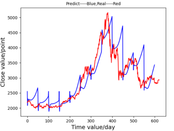
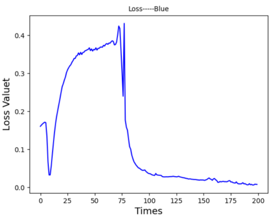
Figure 8. Prediction Graph From LSTM-Ⅰ Figure 9. Prediction Graph From LSTM-Ⅰ

To refine the model, the learning rate was reduced to 0.0005. This change produced a more responsive prediction graph Figure 10 and a more stable loss curve Figure 11, indicating enhanced sensitivity to subtle changes in stock prices.

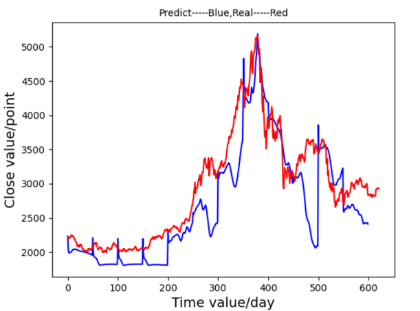
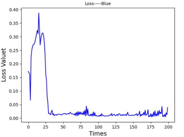
Figure 10. Prediction Graph From LSTM-Ⅱ Figure 11. Prediction Graph From LSTM-Ⅱ

Subsequently, the time step was adjusted from 50 to 20, yielding an improved fit to the actual data with a faster training time of approximately 20 minutes. The resulting prediction graph Figure 12 displayed a closer match to the real stock trend, though minor increases in the loss function Figure 13 suggested further tuning was needed.

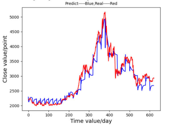
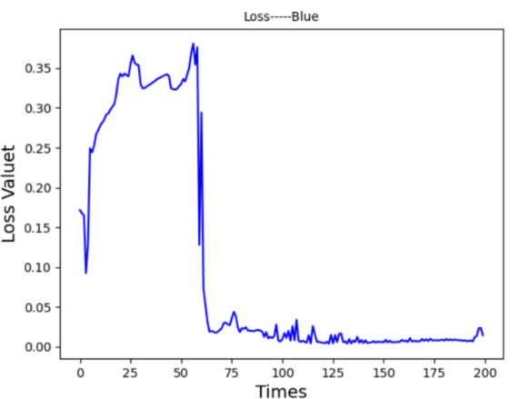
Figure 12. Prediction Graph From LSTM-Ⅲ Figure 13. Prediction Graph From LSTM-Ⅲ

An increase in neurons per LSTM layer, from 10 to 30, provided additional model accuracy for both broader trends and finer details, as seen in the prediction graph Figure 14. The adjusted model also achieved a quicker and more consistent loss function decline Figure 15. Although the increased neuron count improved the model’s fitting ability, it introduced a risk of overfitting. Therefore, additional optimization focused on configuring the number of hidden layers.

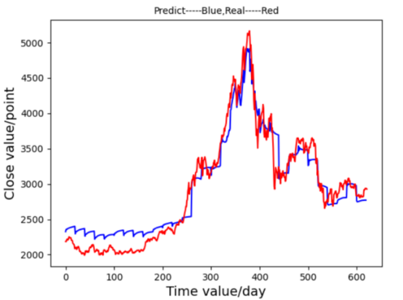
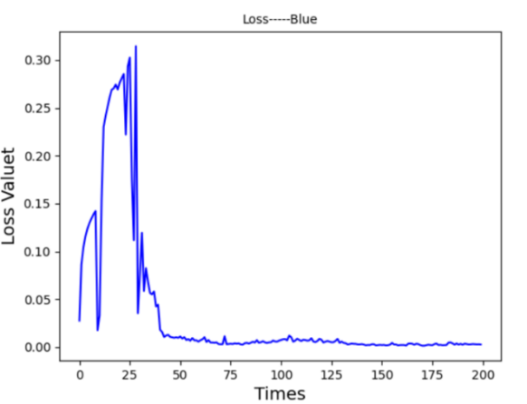
Figure 14. Prediction Graph From LSTM-Ⅳ Figure 15. Prediction Graph From LSTM-Ⅳ

Adjusting the number of hidden layers revealed that too few layers caused oscillations in the loss function, while too many layers increased overfitting risk and training time. By reducing hidden layers from 14 to 5, the model achieved efficient training within 8 minutes and 45 seconds. This final configuration provided highly accurate predictions, as illustrated in Figure 16, with the loss function rapidly decreasing and stabilizing at a low value of 0.00067, as shown in Figure 17. The optimized model demonstrated a close alignment between the predicted and actual stock values, underscoring the model’s generalization and fit for stock prediction.

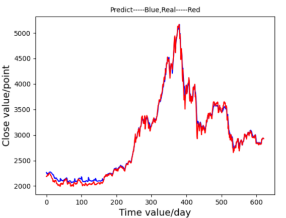
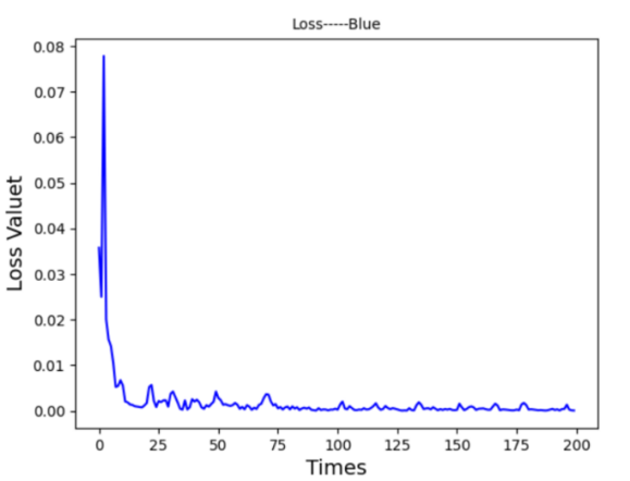
Figure 16. Prediction Graph From LSTM-Ⅴ Figure 17. Prediction Graph From LSTM-Ⅴ

To sum up, this LSTM-based model underwent systematic optimization through adjustments to the learning rate, time steps, neuron count, and hidden layers, resulting in an efficient and accurate stock prediction system. The final configuration, depicted in Figures 16 and 17, highlights LSTM's capacity to capture complex temporal dependencies and enhance forecasting precision, making it well-suited for applications in stock market analysis where accurate trend prediction is essential.

4. Results Analysis

With the purpose of creating a neural network system for predicting stocks, this study compared the prediction ability of MLP, RNN, GRU, and LSTM (without optimization) for the series of stock data, and optimized and adjusted LSTM after determining that LSTM is the most suitable network due to the comparison shown in Table 1.

Table 1. Comparision of Performance in Different Models

The running environment used in this study is the Win10 system, the GPU of NVIDIA GeForce RTX3060, the Python version 3.7.7, cuda in version 11.1, cuDNN in version 8.0.5, and the TensorFlow GPU version 2.4.1. In this environment, the original training time required about 22 minutes and the value of the loss function was 0.34529. After reducing the learning rate from 0.001 to 0.0005, and adjusting the time step from 50 to 20, we reduced each hidden layer neuron. From the time of the final training, the model was iterated 200 times in 8 minutes and 45 seconds, and the training prediction image and loss function image are shown in Figures 15 and 16 respectively, and the value of the final loss function is reduced to 0.00067.

This paper presents findings from debugging experiments that highlight the effectiveness of LSTMnetworks in stock price forecasting. LSTM models capture temporal dependencies through state memory, mitigating gradient explosion and vanishing issues common in traditional RNNs, thus making them highly suited for complex time-series predictions. Optimizing the initial LSTM model requires careful tuning based on dataset characteristics. Key steps include aligning network architecture with task requirements, normalizing data, and adjusting learning rates to stabilize output fluctuations. Overfitting and underfitting issues can be addressed by modifying neuron counts or hidden layers. These refinements, tailored to dataset properties and objectives, significantly improve model performance. Ultimately, the system demonstrates high accuracy in predicting stock trends, showcasing the value of neural networks in stock market analysis and enhancing their practical application in financial forecasting.

5. Conclusion

In summary, after an extensive review of neural network methodologies, this paper presents a sophisticated stock prediction system founded on the LSTM neural network architecture. Comparative analysis reveals LSTM's pronounced suitability for temporally dependent data, such as stock prices. Unlike conventional RNNs, which face issues of gradient explosion and vanishing, LSTM enhances temporal stability by selectively retaining crucial historical information, thereby optimizing memory function over time.

Following the construction of the LSTM model, key parameters—including the number of hidden layers, learning rate, and time steps—were rigorously refined to align with dataset characteristics, facilitating more efficient training, heightened predictive precision, and an optimal loss function value of 0.00067. Despite the model's proven predictive strength, certain limitations were identified. The complex architecture of LSTM networks can hinder computational efficiency, making parameter adjustments challenging and time-intensive. Furthermore, the model is less suited to parallel processing tasks, limiting its adaptability in some computational contexts. Future research directions may further investigate LSTM's applications in time-sensitive domains such as machine translation, conversational AI, and text recognition, where mastering temporal dependencies remains imperative.

References

[1]. A. Graves, “Sequence transduction with recurrent neural networks,” in ICML Representation Learning Work sop, 2012.
[2]. Barak A. Pearlmutter. Gradient calculations for dynamic recurrent neural networks: A survey. Neural Networks, IEEE Transactions on, 6(5): 1212–1228, 1995.
[3]. Liu, X., Wu, Y., Luo, M., & Chen, Z. (2024). Stock price prediction for new energy vehicle companies based on multi-source data and hybrid attention structure. Expert Systems With Applications, 255, 124787. https://doi.org/10.1016/j.eswa.2024.124787
[4]. S. Mandal and N. Prabaharan, “Ocean wave prediction using numerical and neural network models,” The Open Ocean Engineering Journal, vol. 3, no. 1, 2010.
[5]. M. Bodén (2001. November 13th). A Guide to Recurrent Neural Networks and Backpropagation, from https://www.researchgate.net/publication/2903062
[6]. S.D. Yang, Y. Zhou and X.Y. Yu(2020). LSTM and GRU neural network performance comparison study
[7]. S. Fan, N. Xiao, and S. Dong, “A novel model to predict significant wave height based on long short-term memory network,” Ocean Engineering, vol. 205, p. 107298, 2020.
[8]. A.T. Sukanda, D. Adytia. (2022) Wave Forecast using Bidirectional GRU and GRU Method Case Study in Pangandaran, Indonesia
[9]. Y. Zhang, G. Chen, D. Yu, K. Yaco, S. Khudanpur, and J. Glass, “Highway long short-term memory rnns for distant speech recognition”
[10]. Z.C. Lipton & J. Berkowitz (2015, June 5th) A Critical Review of Recurrent Neural Networks for Sequence Learning
[11]. Werbos, P. J. (1988). Generalization of backpropagation with application to a recurrent gas market model. Neural Networks, 1.
Cite this article
Hu,J. (2024). A High-Performance Stock Prediction System Leveraging LSTM Neural Networks. Applied and Computational Engineering,114,65-72.
Data availability
The datasets used and/or analyzed during the current study will be available from the authors upon reasonable request.
Disclaimer/Publisher's Note
The statements, opinions and data contained in all publications are solely those of the individual author(s) and contributor(s) and not of EWA Publishing and/or the editor(s). EWA Publishing and/or the editor(s) disclaim responsibility for any injury to people or property resulting from any ideas, methods, instructions or products referred to in the content.
About volume
Volume title: Proceedings of the 2nd International Conference on Machine Learning and Automation
© 2024 by the author(s). Licensee EWA Publishing, Oxford, UK. This article is an open access article distributed under the terms and
conditions of the Creative Commons Attribution (CC BY) license. Authors who
publish this series agree to the following terms:
1. Authors retain copyright and grant the series right of first publication with the work simultaneously licensed under a Creative Commons
Attribution License that allows others to share the work with an acknowledgment of the work's authorship and initial publication in this
series.
2. Authors are able to enter into separate, additional contractual arrangements for the non-exclusive distribution of the series's published
version of the work (e.g., post it to an institutional repository or publish it in a book), with an acknowledgment of its initial
publication in this series.
3. Authors are permitted and encouraged to post their work online (e.g., in institutional repositories or on their website) prior to and
during the submission process, as it can lead to productive exchanges, as well as earlier and greater citation of published work (See
Open access policy for details).