


1. Introduction
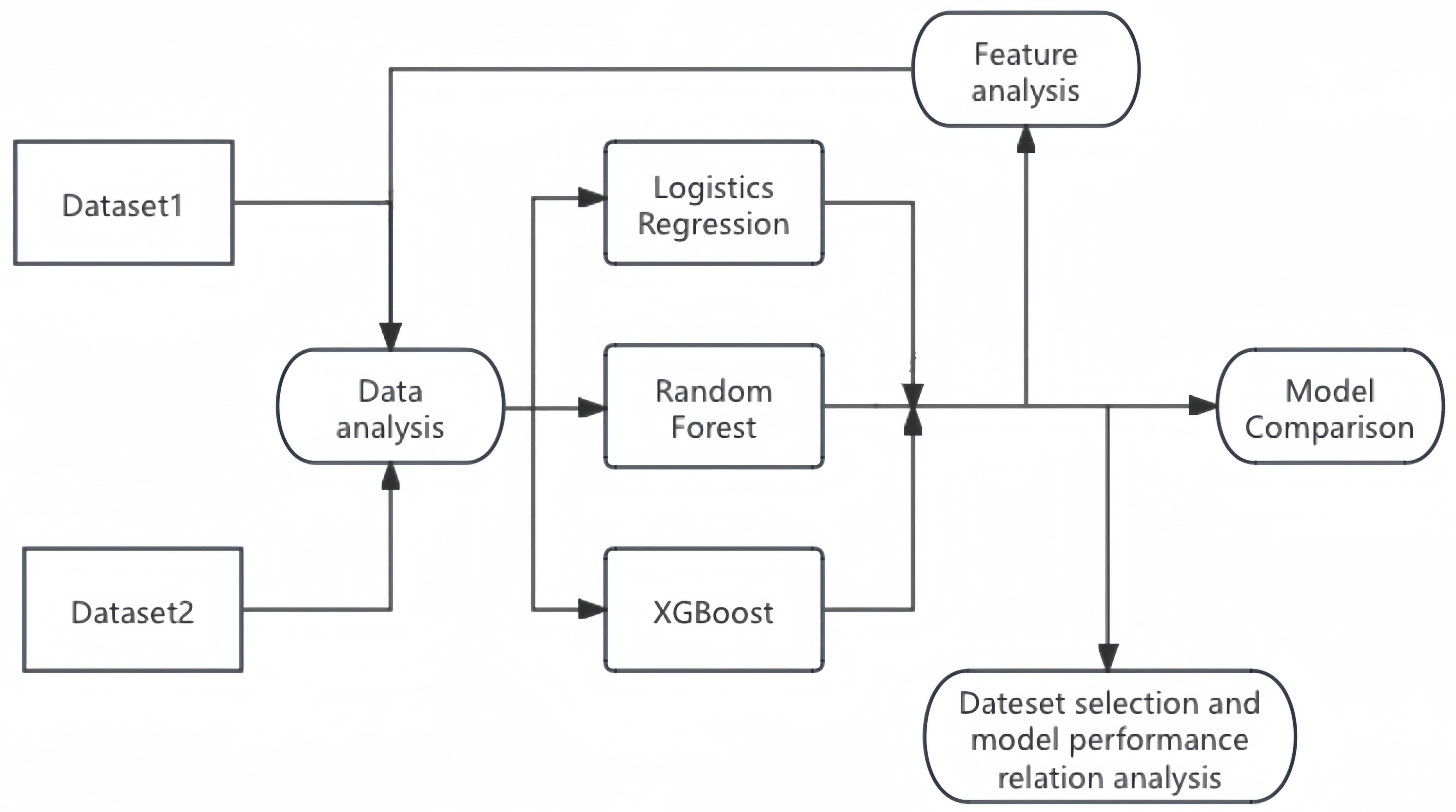
In the field of diabetes prediction, numerous methods have been applied by researchers. The effectiveness of the predictions on the dataset varies from model to model. While reviewing the papers, it was found that each paper used a different dataset for the study, but no paper was found that would use more than one dataset for the study. Therefore, this study considers using two different datasets for the study to see if there is a significant effect of different datasets on the machine learning prediction effect. In this study, it was decided to use the method of meta-analysis. Aishwarya Mujuumdar and Dr.Vaidehi V [1] studied the effects of various machine learning models in diabetes prediction and compared the results. Accuracy and F1 scores were used to evaluate the model. Studies have shown that Logistic Regression has the best prediction effect. Zou et al. [2] used decision trees, random forests, and neural network models to make predictions, and used principal component analysis to extract important features. It is concluded that the prediction effect of random forest is the best. Researchers such as Isfafuzzaman Tasin [3] also compared and analyzed the prediction effect through multiple machine learning models. The conclusion reached was that XGBoost's metrics were the best. M. ABU SAYEED ET AL. [4] used a stepwise logistic regression method for their studies. Therefore, in this study, three models of logistic regression, random forest, XGBoost and two different datasets were used to predict diabetes and compare their performance. In pathology, factors such as BMI and blood glucose indicators are common factors influencing diabetes. Ian H. de Boer et al. [5] have mentioned hypertension as a strong, modifiable risk factor for macrovascular and microvascular complications of diabetes. Zihui Yan et al. [6] identified differences in risk factors for diabetes in different age groups. Natallia Gray et al. [7] found that overweight and obesity are major factors contributing to type 2 diabetes and its complications. Researchers such as Rita R.Kalyani [8] mentioned in their study that adults with diabetes have a higher prevalence of heart disease, regardless of definition, than adults without diabetes. There is a significant relationship between diabetes and heart disease. Therefore, this study hypothesized that age, BMI, high blood pressure, and the presence or absence of heart disease are key factors that influence diabetes prediction. The meta-analysis approach was used for the study, combining the predictive tools used in several papers. The papers referenced all chose a single dataset for prediction, so this study wanted to explore the generalizability of machine learning models to the dataset. We evaluated the datasets by training them independently, using one dataset as a training set and the other as a test set, as well as attempting to merge the two datasets for a generalizability study in order to explore the factors indicative of diabetes prediction models with real-world relevance. Two different datasets were selected and three different learning methods were chosen. It is hoped to compare the prediction effects of different machine learning models on different datasets, to find out the main features affecting the prediction of diabetes, and to select the model with the best prediction effect. At the same time, this study also hopes to investigate the different data and whether there is a significant effect on the prediction effect of the models.
2. Methodology
2.1. Meta-analysis
Meta-analysis is a statistical analysis technique that improves statistical power and robustness of effect estimates by encompassing multiple different studies addressing the same scientific question. In the field of machine learning, meta-analysis can help determine which machine learning model performs best across different studies and datasets, and analyze the impact of dataset selection on model performance. It can also reveal the most important predictive features of diabetes, providing insights into disease mechanisms and guiding future research. Meta-analysis helps resolve contradictions in individual studies, improve estimate accuracy, and identify trends. This study employs meta-analysis methods to train and evaluate three machine learning approaches using two different diabetes datasets, effectively enhancing the accuracy of the research conclusions.
2.2. Model Introduction
Logistic Regression In order to maximize the probability that random data points will be correctly classified, maximum likelihood estimation is used, and likelihood functions are used, which are used to solve binary classification problems.
Random Forest In order to address the inherent flaws of a single model, use the bootstrap method to generate multiple training sets, build a decision tree for each training set, randomly select a part of the features, find the optimal solution, and apply it to the nodes for splitting.
XGBoost Multiple trees are used to make decisions together, and the result of each tree is the difference between the target value and the predicted effect of all previous trees, and all the effects are added up to arrive at the final result. The basic steps are: learn the t-tree, define the objective function, use Taylor's formula to expand, define a tree and its complexity, group the leaf nodes, and finally score the tree structure.
2.3. Model Evaluation Methodology
In this study, the confusion matrix, accuracy, F1 score, ROC curve with AUC value are mainly used to assess the effectiveness of model assessment. The following is an explanation of the various assessment metrics:
Table 1: Confusion Matrix
| Freq | class one actual | class two actual |
|---|---|---|
| class two predicted | FP | TN |
| class one predicted | TP | FN |
TP (True Positives) True examples, positive examples are predicted to be true (predictions are positive examples and are actually positive examples); FP (False Positives) False positives, negative examples are predicted to be true (predictions are positive but are actually negatives); FN (false negatives) False negatives, positive predictions are false (predictions are negative but are actually positives); TN (True Negatives) True negatives, negative predictions are false (predictions are negative and are actually negatives). Accuracy The ratio of the number of correct predictions to the total number of positive and negative examples.
F1 score Precision, refers to the proportion of samples with a predicted value of 1 and a true value of 1 to all samples with a predicted value of 1. Recall, also known as recall, refers to the proportion of samples with a predicted value of 1 and a true value of 1 to all samples with a true value of 1. \[ \begin{array}{ccc} P = \frac{TP}{TP + FP} & R = \frac{TP}{TP + FN} & F1 = \frac{2P \cdot R}{P + R} \end{array} \] ROC curve evaluation model The Receiver Operating Characteristic (ROC) curve is a comprehensive indicator that is used to express the relationship between sensitivity and specificity. The ROC curve elucidates the interplay between sensitivity and specificity through graphical representation. It is a plot with the false positive rate on the horizontal axis and the true positive rate on the vertical axis. By setting multiple different thresholds for continuous variables, a series of sensitivity and specificity values are calculated. The ROC curve is then plotted with sensitivity on the vertical axis and specificity on the horizontal axis. The larger the area under the curve (AUC), the higher the diagnostic accuracy.
3. Identifying The Key Feature Factors of Diabetes Prediction
3.1. Data analysis
Two different datasets were collected for this study, the diabetes prediction dataset from medical and demographic statistics [9] and the diabetes health indicator dataset from CDC statistics [10], which were named dataset 1 and dataset 2, respectively. The datasets chosen for this study are large in number, dataset 1 contains 100,000 data, and dataset 2 contains about 250,000 data. dataset 1 contains factors such as gender, age, and blood glucose, and dataset 2 contains factors such as hypertension, blood lipids, and heart disease.
Table 2: Dataset 1 Data Characteristics
| Variable Name | Description |
|---|---|
gender |
Male or female |
age |
Specific age |
hypertension |
Whether you have high blood pressure |
heart\_disease |
Whether you have heart disease |
smoking\_history |
The status category of smoking |
BMI |
Body Mass Index |
HbA1c\_level |
Glycosylated hemoglobin level |
blood\_glucose\_level |
Blood sugar level |
Table 3: Dataset 2 Feature Interpretation
| Variable Name | Description |
|---|---|
HighBP |
High Blood Pressure |
HighChol |
High blood cholesterol |
CholCheck |
Whether cholesterol check was done in the past 5 years |
BMI |
Body Mass Index |
Smoker |
Have you smoked at least 100 cigarettes in your life |
Stroke |
Have you ever had a stroke |
HeartDiseaseorAttack |
Have you had a heart attack |
PhysActivity |
Have you been physically active in the past 30 days (excluding work) |
Fruits |
Eat 1 or more fruits per day |
Veggies |
Eat 1 or more vegetables per day |
HvyAlcoholConsump |
Whether or not you are an alcoholic |
AnyHealthcare |
Whether you have any health insurance |
NoDocbcCost |
Whether or not you have expenses for doctor's visits |
GenHlth |
Human health status |
MentHlth |
Number of mental health days in 30 days |
PhysHlth |
Number of physical health days in 30 days |
Diffwalk |
Whether you have difficulty walking |
Sex |
Male or Female |
Age |
Age range |
Education |
What is the highest grade or year of school you completed |
Income |
Income level |
Dataset 1 contains textual data. The gender characteristics were originally textual, and this study defines "Female" as 0 and "Male" as 1. The smoking\_history was also originally textual and contains multiple categories. This study defines "never" as 0 and "1" for the rest. The data were checked for missing values and duplicates, and duplicates were removed. For Dataset 2, all variables are of numeric type. The data were checked for missing values and duplicates, and duplicates were removed. The Pearson and Spearman correlation coefficients are visualized for the two processed datasets respectively.
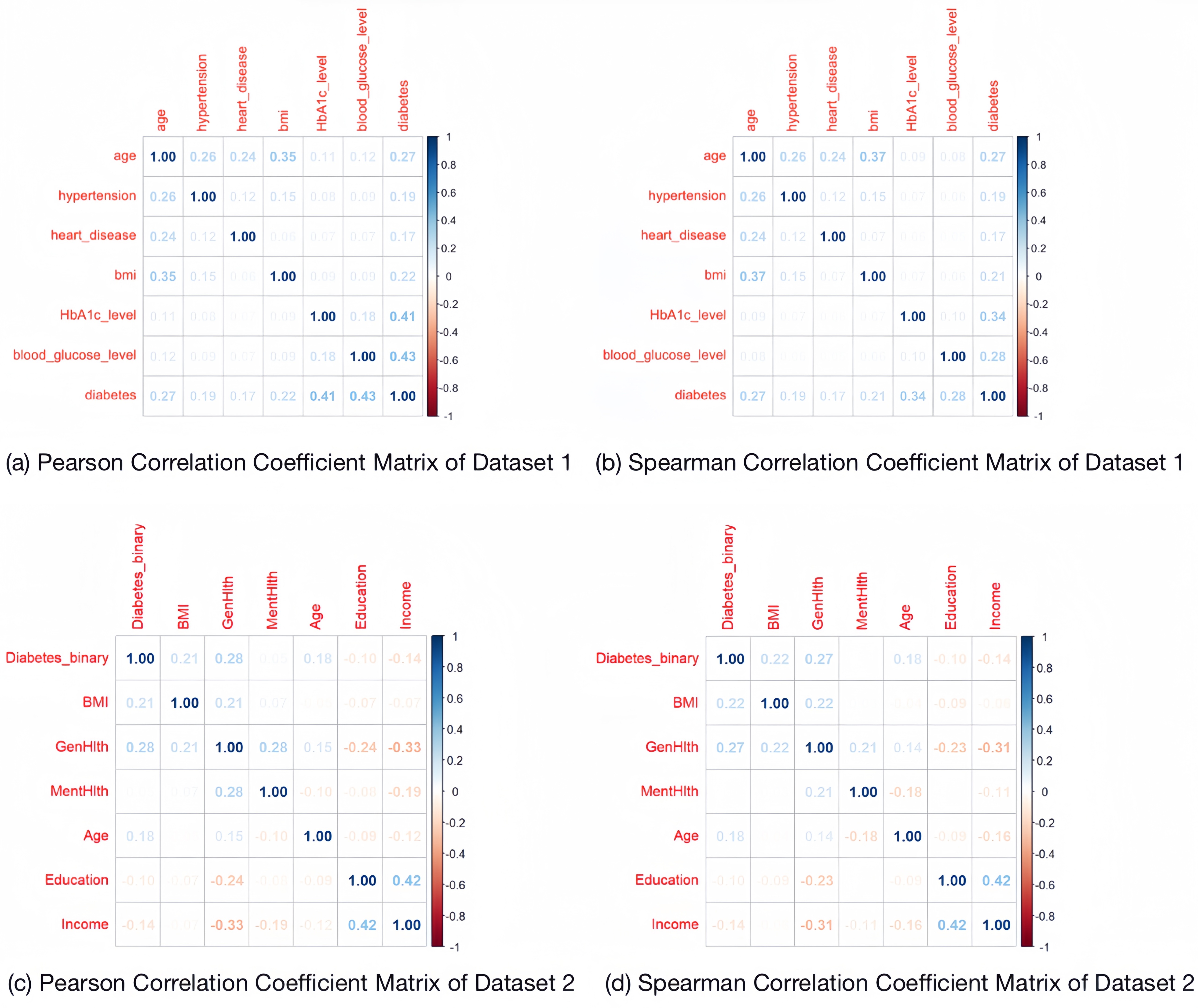
From the coefficient matrix, it can be seen that the values of their correlation coefficients are all low, so the multicollinearity between the features is not obvious.
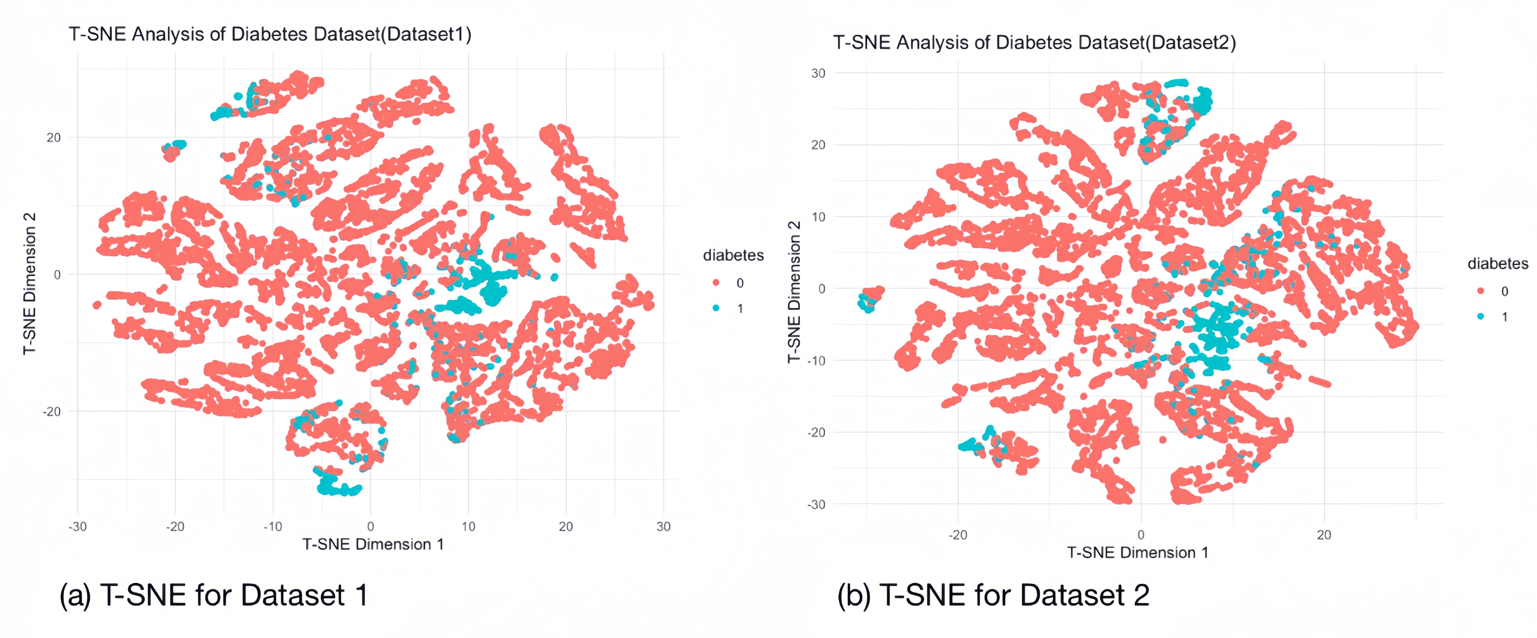
3.2. T-distributed Stochastic Neighbor Embedding
The T-SNE technique is used in the visualisation of diabetes datasets to display high dimensional data, providing a location in 2D space for each data point. It helps to model the features of high-dimensional objects into two-dimensional space so that similar objects tend to cluster together, while dissimilar objects are modelled as more distant points. We performed a sampling T-SNE analysis (10,000 randomly selected samples) on each of the two diabetes datasets to separate out the samples representing diseased and non-diseased individuals, and the clustering of the samples of diabetic patients is evident in the images, which suggests that our datasets can be separated on the basis of feature factors.
3.3. Machine Learning Training and Evaluation
We evaluated the training of two datasets using three machine learning methods respectively, with whether or not they have diabetes as the target variable (1: diabetic, 0: normal) and various data indicators as the feature factors, and the results of the evaluations are as follows:
Table 4: Comparison of Accuracy, Confidence Intervals, and F1 Scores for Different ML Models on Two Datasets
| ML\textbackslash Dataset | Dataset1 (100k) | Dataset2 (250k) |
|---|---|---|
| Logistics Regression | \begin{tabular}[c]{@{}c@{}}Accuracy: 0.9338 | |
| 95% CI: (0.9301, 0.9373) | ||
| F1 Score: 0.964696435229 |
& \begin{tabular}[c]{@{}c@{}}Accuracy: 0.8476
95% CI: (0.8443, 0.8509)
F1 Score: 0.917008902077151\end{tabular}
\hline
Random Forest & \begin{tabular}[c]{@{}c@{}}Accuracy: 0.971
95% CI: (0.9627, 0.9779)
F1 Score: 0.984298863021115\end{tabular} & \begin{tabular}[c]{@{}c@{}}Accuracy: 0.847
95% CI: (0.8305, 0.8625)
F1 Score: 0.914763231197772\end{tabular}
\hline
XGBoost & \begin{tabular}[c]{@{}c@{}}Accuracy: 0.9685
95% CI: (0.9659, 0.971)
F1 Score: 0.98283839981257\end{tabular} & \begin{tabular}[c]{@{}c@{}}Accuracy: 0.8525
95% CI: (0.8492, 0.8557)
F1 Score: 0.918056597835823\end{tabular}
\hline
\end{tabular}
3.4. Feature Factors Analysis
Permutation feature importance (PMI) is a technique in machine learning used to assess the importance of different features in a predictive model. The basic idea is to randomly shuffle or rank the values of specific features while keeping other variables constant in order to measure the degree of degradation in model performance. IncNodePurity, or increase in node purity, is measured by the sum of squares of residuals and represents the effect of each variable on the heterogeneity of observations at each node of the classification tree, thus comparing the importance of the variables. By training two different diabetes datasets using three machine learning methods, we take Permutation feature importance (PMI) and IncNodePurity as metrics to analyze the key feature factors corresponding to different machine learning for the two datasets: Logistic Regression Combining the results of the two datasets, we conclude that for Logistic Regression, for dataset 1, blood glucose level, glycated haemoglobin level, age, and BMI are the predictors of the main feature factors. For dataset 2, human health status, hypertension, age, BMI, high cholesterol, gender, cholesterol screening, and heart disease were the main predictive features. Among the key in features common to both models were BMI, age, hypertension, and heart disease. Random Forest Combining the results of the two datasets, we conclude that for Random Forest, for dataset 1, blood glucose level, glycated haemoglobin level, age, and BMI are the predictors of the main feature factors. For dataset 2, age, BMI, income, human health status, education, mental health status, and hypertension were the main predictive features. Among the key features common to both models were BMI, age, and hypertension. XGBoost Combining the results of the two datasets, we conclude that for XGBoost, for dataset 1, blood glucose level, glycated haemoglobin level, age, and BMI are the predicted main feature factors. For dataset 2, high blood pressure, high cholesterol, BMI, age, human health status, income, physical health status, mental health status, and heart disease are the main predictive features. Among the key features common to both models were BMI, age, hypertension, and heart disease.
Table 5: Rank of Feature Importance across ML (Dataset 2)
| Features\textbackslash ML | LR | RF | XGBoost |
|---|---|---|---|
| HighBP | 2 | 8 | 1 |
| HighChol | 5 | 9 | 5 |
| CholCheck | 7 | 21 | 13 |
| BMI | 3 | 1 | 3 |
| Smoker | 18 | 10 | 18 |
| Stroke | 11 | 18 | 16 |
| HeartDiseaseorAttack | 8 | 14 | 9 |
| PhysActivity | 12 | 13 | 17 |
| Fruits | 16 | 11 | 20 |
| Veggies | 14 | 15 | 15 |
| HvyAlcoholConsump | 21 | 20 | 10 |
| AnyHealthcare | 19 | 19 | 21 |
| NoDocbcCost | 13 | 17 | 19 |
| GenHlth | 1 | 4 | 2 |
| MentHlth | 20 | 7 | 8 |
| PhysHlth | 15 | 5 | 7 |
| Diffwalk | 9 | 16 | 14 |
| Sex | 6 | 12 | 12 |
| Age | 4 | 2 | 4 |
| Education | 17 | 6 | 11 |
| Income | 10 | 3 | 6 |
Table 6: Rank of Feature Importance across ML (Dataset 1)
| Features\textbackslash ML | LR | RF | XGBoost |
|---|---|---|---|
| gender | 7 | 8 | 7 |
| age | 3 | 4 | 3 |
| hypertension | 5 | 5 | 5 |
| heart\_disease | 6 | 6 | 6 |
| smoking\_history | 8 | 7 | 8 |
| BMI | 4 | 3 | 4 |
| HbA1c\_level | 2 | 1 | 1 |
| blood\_glucose\_level | 1 | 2 | 2 |
We picked the main feature factors common to each machine learning method in both datasets (for Logistics Regression we picked BMI, age, hypertension, heart disease as the key feature factors, for Random Forest we picked BMI, age, hypertension as the key feature factors, and for XGBoost we picked BMI, Age, Hypertension, Heart Disease as the key feature factors) and re-train the two datasets, evaluation is shown in table [???]. The prediction results show that all three machine learning methods perform well according to the shared key feature factors. Therefore we synthesize the key feature factors corresponding to the three machine learning and conclude: For the diabetes prediction model, age, BMI, high blood pressure, and heart disease play a key role in the prediction. Of course, even though age, BMI, high blood pressure, and heart disease are common feature factors that have an important impact on diabetes prediction, for each different dataset, there are usually unique feature factors that also play an important role in prediction (e.g., blood glucose level and glycated haemoglobin level in dataset 1), and in the following, we exclude the above four common feature factors from the two datasets. After excluding the above four shared feature factors, we will use the machine learning method to train and evaluate the two datasets again, and compare the evaluation results with the evaluation results using only the above four shared feature factors (shown in table [???]), and we can find that the shared feature factors have a certain enhancement effect in the prediction of dataset 2, but for dataset 1, its specific feature factors also play the same role. However, as the most prevalent feature factors for predicting diabetes, age, BMI, hypertension, and heart disease are widely present in various datasets, and their excellent indicative roles have a significant impact in the field of diabetes prediction.
3.5. Analysis of Merged Datasets
In real-world scenarios, the training set and test set of a model often originate from different datasets, and usually we first use the open-source sample data of diabetes patients from public hospitals for training, and test it with the unpublished patient data from private hospitals to evaluate the model's performance. To further explore the generalizability of the four feature factors, we try to evaluate the model's performance by training with three machine learning methods using one dataset as the training set and the other dataset as the test set, the result is shown in table [???].
Table 7: Model Performance on One Dataset as Train Set and Another Dataset as Test Set
| ML\textbackslash Dataset | Dataset 1 as train set | Dataset 2 as train set |
|---|---|---|
| Dataset 2 as test set | Dataset 1 as test set | |
| Logistics Regression | \begin{tabular}[c]{@{}c@{}}Accuracy: 0.845 | |
| 95% CI: (0.8406, 0.8494) | ||
| F1 Score: | ||
| 0.915439717645093 |
& \begin{tabular}[c]{@{}c@{}}Accuracy: 0.786
95% CI: (0.7812, 0.7907)
F1 Score:
0.880125458996328\end{tabular}
\hline
Random Forest & \begin{tabular}[c]{@{}c@{}}Accuracy: 0.8485
95% CI: (0.844, 0.8528)
F1 Score:
0.917680327698418\end{tabular} & \begin{tabular}[c]{@{}c@{}}Accuracy: 0.7861
95% CI: (0.7813, 0.7908)
F1 Score:
0.880230935403086\end{tabular}
\hline
XGBoost & \begin{tabular}[c]{@{}c@{}}Accuracy: 0.8472
95% CI: (0.8428, 0.8515)
F1 Score:
0.915631076168738\end{tabular} & \begin{tabular}[c]{@{}c@{}}Accuracy: 0.7845
95% CI: (0.7798, 0.7892)
F1 Score:
0.877651529840617\end{tabular}
\hline
\end{tabular}
The results of the model evaluation show that by selecting the four key features of BMI, age, heart disease and high blood pressure, the model trained on one dataset still performs well in the test on another dataset. This suggests that these four features not only have an important predictive role in the original dataset, but also show good predictive effects on different datasets with good generalization ability, proving that they are important factors with significant indications in diabetes prediction.
Further research, in order to test the role of feature factors such as age, BMI, hypertension, and heart disease in the prediction of diabetes under a broader relevance, we tried to merge the two datasets, keeping only the common feature factors of age, BMI, hypertension, and heart disease. First we performed a sampling T-SNE analysis (100,000 randomly selected samples) on the merged dataset:
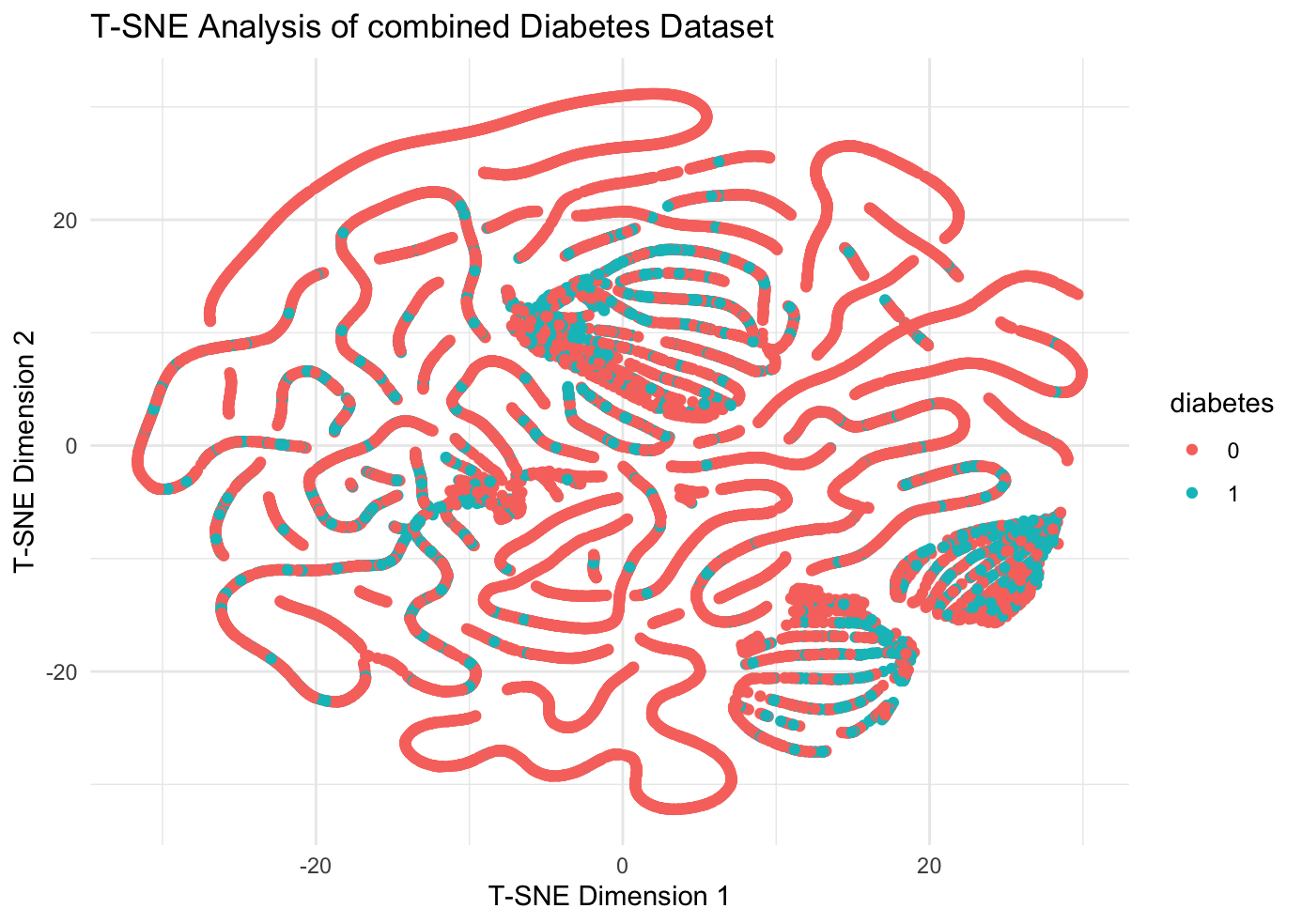
It can be observed that the merged dataset still has significant clustering phenomenon, and then the three machine learning methods are used to train and the results of evaluation are produced in table [???]. The study data show that machine learning prediction models with age, BMI, hypertension, and heart disease feature factors have good performance in the combined dataset, which implies that indicators such as age, BMI, hypertension, and heart disease play an important role in the prevention and diagnosis of diabetes, and the conclusions are of great practical significance.
Table 8: Machine Learning Evaluation Results With and Without Shared Feature and Combined Dataset
\resizebox{\textwidth}{!}{%
| ML\textbackslash Dataset | Dataset1(100k) | Dataset1(100k) | Dataset2(250k) | Dataset2(250k) | Combined Dataset(350k) |
|---|---|---|---|---|---|
| Only with shared features | Without shared features | Only with shared features | Without shared features | Only with shared features | |
| Logistics Regression | Accuracy: 0.9047 | Accuracy: 0.9265 | Accuracy: 0.8442 | Accuracy: 0.8461 | Accuracy: 0.7996 |
| 95% CI: (0.9003, 0.9088) | 95% CI: (0.9226, 0.9302) | 95% CI: (0.8408, 0.8475) | 95% CI: (0.8428, 0.8494) | 95% CI: (0.7906, 0.8085) | |
| F1 Score: 0.949936467598475 | F1 Score: 0.960955128388221 | F1 Score: 0.915358943406944 | F1 Score: 0.916515962790918 | F1 Score: 0.887736732195579 | |
| Random Forest | Accuracy: 0.9085 | Accuracy: 0.971 | Accuracy: 0.841 | Accuracy: 0.8365 | Accuracy: 0.6825 |
| 95% CI: (0.895, 0.9208) | 95% CI: (0.9627, 0.9779) | 95% CI: (0.8242, 0.8568) | 95% CI: (0.8196, 0.8525) | 95% CI: (0.6616, 0.7029) | |
| F1 Score: 0.952056588944197 | F1 Score: 0.984298863021115 | F1 Score: 0.913633894622488 | F1 Score: 0.9093585844623 | F1 Score: 0.645053102291783 | |
| XGBoost | Accuracy: 0.905 | Accuracy: 0.9686 | Accuracy: 0.8464 | Accuracy: 0.8457 | Accuracy: 0.7858 |
| 95% CI: (0.9007, 0.9092) | 95% CI: (0.966, 0.9711) | 95% CI: (0.8431, 0.8497) | 95% CI: (0.8424, 0.849) | 95% CI: (0.7765, 0.7948) | |
| F1 Score: 0.949846643189822 | F1 Score: 0.982938954123079 | F1 Score: 0.91597339753522 | F1 Score: 0.9154882030531982 | F1 Score: 0.877507531780439 |
% }
4. Machine Learning Effectiveness and Dataset Selection Correlation Analysis
Friedman test is a non-parametric statistical method for comparing whether there is a significant difference in the average performance of multiple methods or models on multiple datasets. It does this by ranking the performance on each dataset and then calculating the average ranking and test statistic to determine if the differences between models are significant.
- \(\chi^2_F\) = the Friedman test statistic
- \(k\) = the number of models
- \(n\) = the number of datasets
- \(R_{ij}\) = the rank of the \(j\) -th model on the \(i\) -th dataset
- \(\bar{R_j}\) = the average rank of the \(j\) -th model
\[ \bar{R_j} = \frac{1}{n} \sum_{i=1}^{n} R_{ij} \] \[ \chi^2_F = \frac{12n}{k(k+1)} \left( \sum_{j=1}^{k} \bar{R_j}^2 \right) - 3n(k+1) \] \[ \chi^2_F = \frac{12n}{k(k+1)} \left( \sum_{j=1}^{k} \left( \frac{1}{n} \sum_{i=1}^{n} R_{ij} \right)^2 \right) - 3n(k+1) \] In the following we want to know if the effect of machine learning is linked to the choice of dataset, so we propose the null hypothesis \(H_{0}\) : the effect of machine learning is independent of the choice of dataset. Therefore we use Friedman test (for dataset-model correlation analysis) for table [???]: chi-squared = 1, df = 2, p-value = 0.6065. This means that at 5% level of significance we do not have enough evidence to reject the null hypothesis, i.e., that the effect of the different models (LR, RF and SVM) on the different datasets (Dataset 1 and Dataset 2) there is no significant difference in the performance of different models (LR, RF and SVM) on different datasets (Dataset 2).
5. Comparative Analysis of the Effectiveness of Machine Learning Prediction Models
5.1. Significance Analysis of Model Differences
Kruskal-Wallis test is a non-parametric statistical method for comparing whether the medians of samples from three or more groups are significantly different. It assesses differences between groups by converting the data to rank and calculating the rank sum of the groups, and is a non-parametric alternative to one-way analysis of variance (ANOVA) for data whose distribution is unknown or does not satisfy a normal distribution. \[ H = \frac{12}{N(N+1)} \sum_{i=1}^k \frac{R_i^2}{n_i} - 3(N+1) \] where:
- \( N \) is the total number of observations (total sample size)
- \( k \) is the number of groups
- \( R_i \) is the sum of ranks for the i th group
- \( n_i \) is the number of observations in the i th group
We tried to plot the ROC-AUC plots of each model for each dataset training:
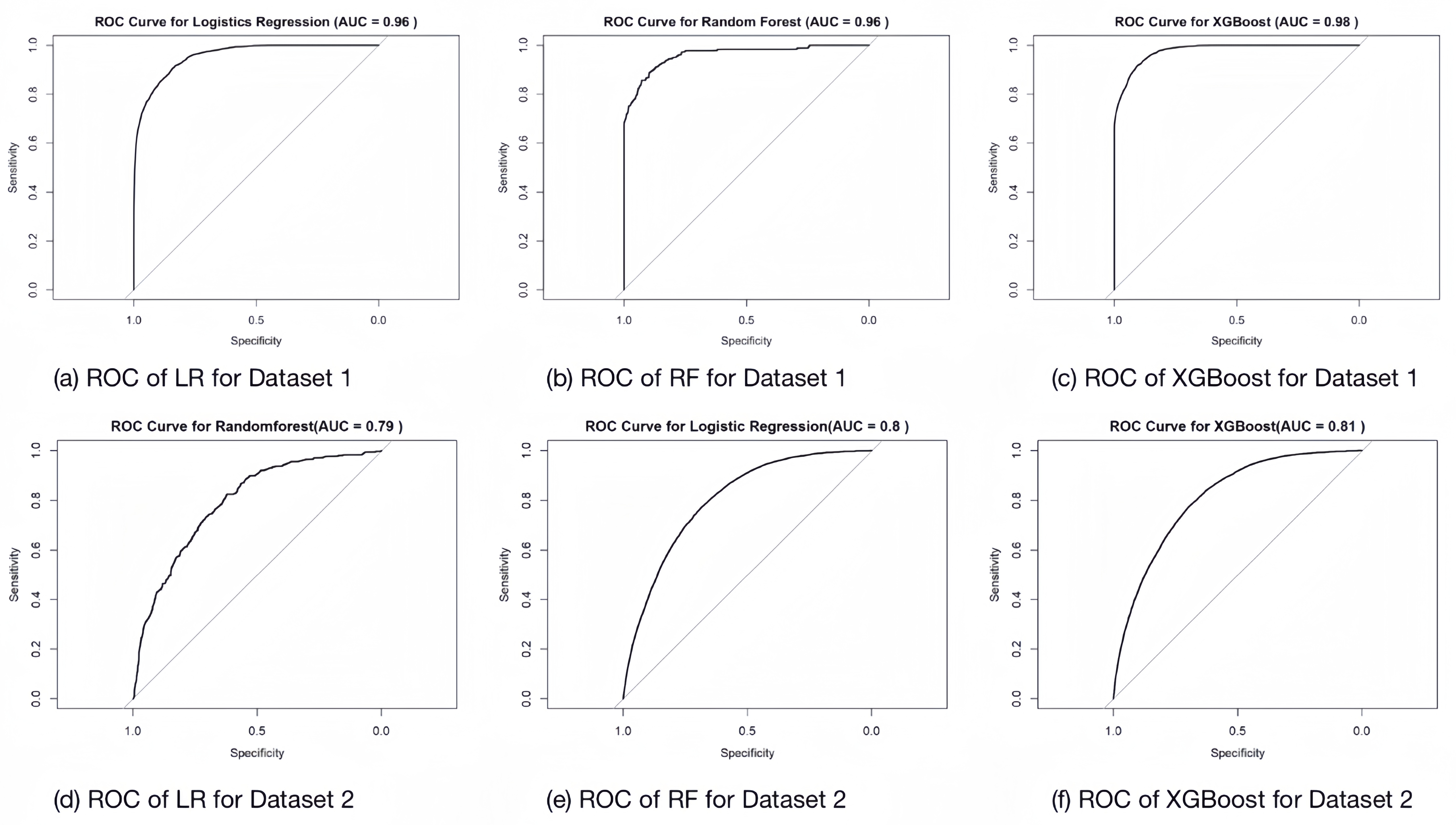
In the following, we want to determine whether there is a significant difference in the performance of different machine learning models. We propose the null hypothesis \(H_{0}\) : there is no significant difference in the performance of these models. We performed the Kruskal-Wallis test for both the F1 score and AUC. The results of the Kruskal-Wallis rank sum test are as follows: For the F1 score: \[ \chi^2 = 3.7143, df = 2, p-value = 0.1561 \] For the AUC: \[ \chi^2 = 0.95588, df = 2, p-value = 0.6201 \] The Kruskal-Wallis test results show that the p-values are all greater than 0.05, indicating that there is not enough evidence to reject the null hypothesis at the 5% significance level. Therefore, we conclude that there is no significant difference in performance between the different models (LR, RF, and XGBoost). As a result, we need to examine the data directly to determine if any nuanced differences exist.
5.2. Comparison of Differences in Machine Learning Prediction Models
We evaluate the difference in the performance of the three models in the two diabetes datasets by plotting the comparison of F1 score and AUC. First, in the comparison of F1 scores, we observe that the F1 scores of both Random Forest and XGBoost are slightly higher than those of Logistic Regression, which suggests that these two models outperform Logistic Regression in terms of the combination of precision and recall. Second, in the comparison of AUC, the mean and maximum values of AUC of XGBoost in both datasets are higher than those of other models. This indicates that XGBoost has the best performance in terms of discriminative ability of the model, which can better distinguish between positive and negative samples.
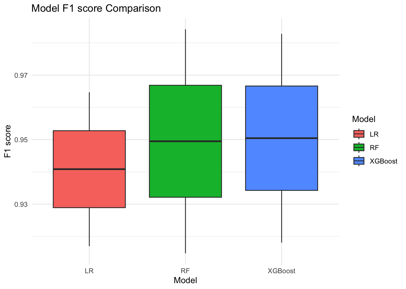
Taken together, we can conclude that XGBoost demonstrated the best prediction performance in the diabetes prediction experiment, with higher accuracy and stability than other models. Therefore, XGBoost is the optimal choice for diabetes prediction in this study.
6. Discussion
The present study has the same limitations. In dataset 2, the feature did not contain a blood glucose indicator, but this feature was prominent in dataset 1. Subsequent studies could take datasets with more comprehensive characteristics and better quality. Future research could try the effects of other models of machine learning, such as neural network models. For the key feature analyzed, using the normal weight group as a control, underweight people had a lower risk of developing pre-diabetes, while overweight and obese people had a higher risk of developing pre-diabetes. Prevalence of diabetes usually increases with age. The higher the blood pressure of a person with hypertension, the higher their risk of developing diabetes. Diabetes and other diseases can interact with each other to cause harmful physical changes to the heart, which can further increase the risk of heart disease. These findings suggest that healthcare practitioners should prioritize the use of XGBoost in predictive modeling and focus on identified key features for effective screening and prevention of diabetes. The robustness of our models across different datasets also ensures their reliable application in different demographic and geographic contexts. Future studies should continue to validate these results and explore additional predictors and machine learning techniques to further improve the performance of diabetes prediction.
7. Conclusion
Our study highlights several key findings in the development of diabetes prediction models using machine learning. First, XGBoost consistently outperformed logistic regression and Random Forest, making it the preferred choice for this task due to its ability to robustly handle complex interactions and reduce overfitting. Second, age, body mass index, hypertension, and cardiovascular disease emerged as the most critical predictive features, highlighting their importance in diabetes risk assessment and the need to develop targeted screening and prevention strategies. Using only the above key factors, the performance of the predictive model can approach or exceed the performance of the full models (with all factors) by more than 95%, indicating that these key factors have a high predictive power in the models. In addition, our hypothesis testing showed that the performance of the machine learning models was independent of the choice of dataset, thus increasing the generalizability of our findings across different populations. This independence supports the broad applicability of these models in a variety of clinical settings. In this study, the same key features from different datasets were combined and analyzed and it was found that the model still had good predictive results. The conclusions drawn are therefore universal.
Acknowledgement
We would like to express our sincere gratitude to Professor Divakaran Liginlal of Carnegie Mellon University for his invaluable guidance and assistance in writing the paper. His advice and support were crucial to the successful conduct of this study.
References
[1]. Mujumdar, A. and Vaidehi, V. (2019). Diabetes prediction using machine learning algorithms. Procedia Computer Science, 165, 292–299.
[2]. Zou, Q., Qu, K., Luo, Y., et al. (2018). Predicting diabetes mellitus with machine learning techniques. Frontiers in Genetics, 9, 515.
[3]. Tasin, I., Nabil, T. U., Islam, S., et al. (2023). Diabetes prediction using machine learning and explainable AI techniques. Healthcare Technology Letters, 10(1–2), 1–10.
[4]. Sayeed, M. A., Ali, L., Hussain, M. Z., et al. (1997). Effect of socioeconomic risk factors on the difference in prevalence of diabetes between rural and urban populations in Bangladesh. Diabetes Care, 20(4), 551–555.
[5]. De Boer, I. H., Bangalore, S., Benetos, A., et al. (2017). Diabetes and hypertension: a position statement by the American Diabetes Association. Diabetes Care, 40(9), 1273–1284.
[6]. Yan, Z., Cai, M., Han, X., et al. (2023). The interaction between age and risk factors for diabetes and prediabetes: a community-based cross-sectional study. Diabetes, Metabolic Syndrome and Obesity, 85–93.
[7]. Gray, N., Picone, G., Sloan, F., et al. (2015). The relationship between BMI and onset of diabetes mellitus and its complications. Southern Medical Journal, 108(1), 29.
[8]. Kalyani, R. R., Everett, B. M., Perreault, L., et al. (2023). Heart Disease and Diabetes. Diabetes in America [Internet].
[9]. Mustafa, I. (2024). Diabetes Prediction Dataset. Retrieved from https://www.kaggle.com/datasets/ iammustafatz/diabetes-prediction-dataset
[10]. Teboul, A. (2024). Diabetes Health Indicators Dataset. Retrieved from https://www.kaggle.com/datasets/ alexteboul/diabetes-health-indicators-dataset
Cite this article
Deng,T.;Luo,W.;Huang,K. (2025). Identifying Key Factors that Influence Diabetes Prediction: A Meta Analysis of Two Datasets and Three Machine Learning Models. Applied and Computational Engineering,132,199-211.
Data availability
The datasets used and/or analyzed during the current study will be available from the authors upon reasonable request.
Disclaimer/Publisher's Note
The statements, opinions and data contained in all publications are solely those of the individual author(s) and contributor(s) and not of EWA Publishing and/or the editor(s). EWA Publishing and/or the editor(s) disclaim responsibility for any injury to people or property resulting from any ideas, methods, instructions or products referred to in the content.
About volume
Volume title: Proceedings of the 2nd International Conference on Machine Learning and Automation
© 2024 by the author(s). Licensee EWA Publishing, Oxford, UK. This article is an open access article distributed under the terms and
conditions of the Creative Commons Attribution (CC BY) license. Authors who
publish this series agree to the following terms:
1. Authors retain copyright and grant the series right of first publication with the work simultaneously licensed under a Creative Commons
Attribution License that allows others to share the work with an acknowledgment of the work's authorship and initial publication in this
series.
2. Authors are able to enter into separate, additional contractual arrangements for the non-exclusive distribution of the series's published
version of the work (e.g., post it to an institutional repository or publish it in a book), with an acknowledgment of its initial
publication in this series.
3. Authors are permitted and encouraged to post their work online (e.g., in institutional repositories or on their website) prior to and
during the submission process, as it can lead to productive exchanges, as well as earlier and greater citation of published work (See
Open access policy for details).
References
[1]. Mujumdar, A. and Vaidehi, V. (2019). Diabetes prediction using machine learning algorithms. Procedia Computer Science, 165, 292–299.
[2]. Zou, Q., Qu, K., Luo, Y., et al. (2018). Predicting diabetes mellitus with machine learning techniques. Frontiers in Genetics, 9, 515.
[3]. Tasin, I., Nabil, T. U., Islam, S., et al. (2023). Diabetes prediction using machine learning and explainable AI techniques. Healthcare Technology Letters, 10(1–2), 1–10.
[4]. Sayeed, M. A., Ali, L., Hussain, M. Z., et al. (1997). Effect of socioeconomic risk factors on the difference in prevalence of diabetes between rural and urban populations in Bangladesh. Diabetes Care, 20(4), 551–555.
[5]. De Boer, I. H., Bangalore, S., Benetos, A., et al. (2017). Diabetes and hypertension: a position statement by the American Diabetes Association. Diabetes Care, 40(9), 1273–1284.
[6]. Yan, Z., Cai, M., Han, X., et al. (2023). The interaction between age and risk factors for diabetes and prediabetes: a community-based cross-sectional study. Diabetes, Metabolic Syndrome and Obesity, 85–93.
[7]. Gray, N., Picone, G., Sloan, F., et al. (2015). The relationship between BMI and onset of diabetes mellitus and its complications. Southern Medical Journal, 108(1), 29.
[8]. Kalyani, R. R., Everett, B. M., Perreault, L., et al. (2023). Heart Disease and Diabetes. Diabetes in America [Internet].
[9]. Mustafa, I. (2024). Diabetes Prediction Dataset. Retrieved from https://www.kaggle.com/datasets/ iammustafatz/diabetes-prediction-dataset
[10]. Teboul, A. (2024). Diabetes Health Indicators Dataset. Retrieved from https://www.kaggle.com/datasets/ alexteboul/diabetes-health-indicators-dataset