1. Introduction

In recent years, reinforcement learning has been applied in many fields, especially deep reinforcement learning. Deep reinforcement learning can complete tasks that humans cannot finish.

Deep reinforcement learning can be divided into three categories, depending on whether the learning is based on a value function, search and supervision, or a strategy gradient. Traditional reinforcement learning can be combined with the deep learning network using these three methods. However, because of the integration of neural networks in deep reinforcement learning, this model of deep reinforcement learning will consume memory and other computing resources. In some complex scenarios, it will take up too much computing resources. Therefore, it is necessary to utilize compression for deep reinforcement learning.

Compression algorithms are required to solve the depth of the neural network needed to calculate force and memory footprint. Compression algorithms can be divided into quantitative and distillation. Pruning is used to influence the distribution of neural networks for model input and output by removing nodes. Distillation compresses a larger network to a much smaller network. Through their realization principle, pruning and distillation only compress the model structure in the forward propagation process. The quantitative method will compress in the forward and back propagation processes of the model at the same time. The training process of deep learning models involves a lot of back propagation training, and the quantitative compression method will compress the model more significantly.

For this project, we selected the Deep Q-Network (DQN) and the modified Deep Deterministic Policy Gradient (DDPG) models to compress the experimental object. DQN is a deep reinforcement learning based on value, and DDPG is based on the strategy. They are two types of comparison methods, and many methods are based on their improvement. We will use Atari games to evaluate the actual effect of enhanced deep reinforcement learning after model compression. By comparing DQN and DDPG models after compression, we can determine the effectiveness of the compression algorithms for different types of deep reinforcement learning.

2. Related work

There are two concepts that are important for this project. First, the theory of reinforcement learning, including traditional methods (Q-learning, policy gradient) and deep reinforcement learning methods (DQN and DDQN). Second, Quantization aware training, which is the theory of quantization for neural networks.

Q-learning is a fundamental concept of reinforcement learning. This method had the best performance of actions for the Markovian domain [1]. The policy gradient method is a function approximation-based method in reinforcement learning and depends on the function approximator [2]. DQN is a convolutional neural network, which is optimized by the Q-learning variant. The images of the game are converted to raw pixels and are used as the input. The network will then output the reward value for next episode training. DQN has achieved good performance with Atari games previously [3].

Although DQN solves problems with high-dimensional observation spaces, it can only handle discrete and low-dimensional action spaces. Many tasks of interest, such as physical control tasks, have continuous (real valued) and high-dimensional action spaces. DQN cannot be directly applied to continuous domains because it relies on finding the action that maximizes the action-value function. The continuous valued case requires an iterative optimization process at every step. DQN presents a model-free and actor-critic based policy gradient method for reinforcement learning. It can solve more than 20 simulated physics tasks, including classic problems such as cartpole swing-up, dexterous manipulation, legged locomotion and car driving [4].

Quantization reduces the complexity of any model by reducing the precision requirements for weights and activations. This approach has many advantages. First of all, it is broadly applicable across a range of models. It also has a smaller model footprint. With 8-bit quantization, the model size can be reduced by a factor of 4, with minimal accuracy loss. It can also use less working memory and cache for activations [5].

Quantization aware training can substantially improve the accuracy of models by modeling quantized weights and activations during the training process. It is suitable for the case of backforward in this experiment.

3. Method

3.1. Overview

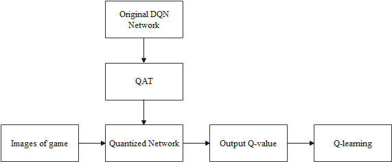
The overview of this project is shown in Figure 1. The DQN is selected and will be quantified by QAT. Every frame of the image from the game will then be inputted into the qualified network for training. Each image will be processed by the agent of the DQN and corresponding Q-value will be outputted to optimize the agent in this training.

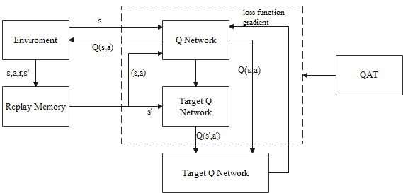
\( TargetQ=r+γmax{a^{ \prime }}Q({s^{ \prime }},{a^{ \prime }};θ) \) (1)

\( L(θ)=E[{(TargetQ-Q(s,a;θ))^{2}}] \) (2)

About the above two formulas, the r means the rewards value, the a is the action value of the agent, and the s means the state of the agent in this leaning, the \( γ \) is the learning rate of this system.

There is a concept called experience pool in this theory of DQN, which describes that the transfer samples (e.g., \( {s_{t}},{a_{t}},{r_{t}},{s_{t+1}} \) ) will be stored in the replay memory, and these samples will be used randomly for training.

The training steps of the DQN are as follows: First of all, the capacity of the experience pool will be initialized as N size. Secondly, parameters of the DQN will be initialized with random values. Thirdly, the loop is started with by initializing s1 and pre-processing the \( {ϕ_{1}}=ϕ({s_{1}}) \) , then creating a loop for random selection for exploration rate \( ∈ \) to get the reward and the target Q-value can be obtained. Finally, the parameters are updated by gradient descent.

3.2. DQN strategy

The structure of the DQN is a convolution neural network. The size of the input is 84 x 84 x 4. This network contains three hidden layers. The first is a convolution layer, which has 16 convolution kernels. The size is 8 x 8, with a step size of 4, and the activation function is ReLU. The size of the output is 20 x 20 x 16. The second layer is also a convolution layer, with 32 x 4 x 4 convolution kernels. The size is 4 x 4, step size is 2, and the activation function is ReLU. The output size is 9 x 9 x 32. The third layer is a full connection layer, with 256 rectifier units and the output size is 256 x 1.

3.3. Quantization

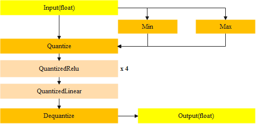
Quantization is achieved by converting common operations into equivalent 8-bit versions. Operations covered include convolution, matrix multiplication, activation functions, pooling operations, and concatenation. The transformation script starts by replacing each known operation with an equivalent quantized version. The operation is then preceded by a subgraph containing a conversion function that converts input from float to 8 bits and output from 8 bits back to float. After the conversion, the input and output are still floating, but the intermediate calculation uses 8 bits.

Quantizing takes the Min and Max from the input, corresponding to the minimum value (0) and maximum value (255) in the quantized input respectively, divides the interval [Min, Max] evenly into 255 cells, and puts the values in the input into the corresponding interval. The reverse quantization operation reverses the above operation. For example, if the maximum input value is 30.0 and the minimum value is -10.0, the quantized values are shown in Table 1.

Table 1. Quantized values.

As shown in Figure 3, in order to quantify the selected CNN network, we will determine the quantization standard by setting the maximum and minimum values, and quantifying four ReLu layers and one linear layer.

4. Results and Analysis

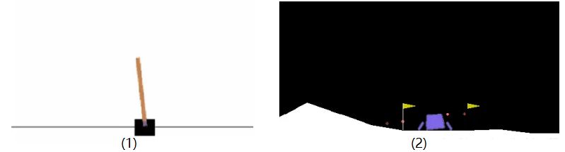
For this project, we used two games to train the two agents of the DQN and the DQN processed by QAT. The first game is called CartPole, which is a game where the player controls a matchstick and tries to keep it vertical by moving its base to the left or right. The second game is called LunarLander, in which the player controls a spaceship, moving it to the left or right so that it lands in the correct place. Screenshots of the two games are shown in Figure 4.

After training the DQN and DQN processed by QAT agents, the memory used was decreased by QAT (Table 2).

Table 2. Memory usage for original DQN and DQN after QAT.

Figure 5 shows the reward trends for CartPole. The first plot is the reward trend for original DQN in the training process, and the second plot is the reward trend for DQN after QAT in the training process.

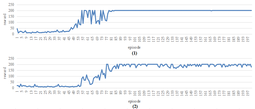
In this process, the two agents were trained for 200 episodes. A reward value of 200 is needed to achieve the expected performance. When the reward is larger than 200, the reward is set to 200. By comparing the two trends, the original DQN reaches the expected performance earlier than DQN after QAT, and the trend of DQN is more stable after reaching the expected performance than DQN after QAT.

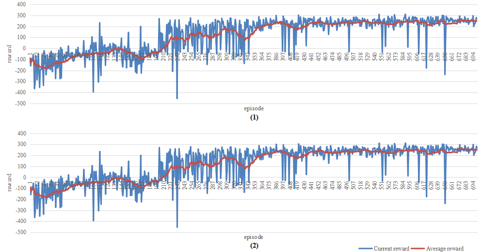
Figure 6 shows the reward trend for LunarLander. The first plot is the reward trend for original DQN in the training process, and the second plot is the reward trend for DQN after QAT in the training process.

In this process, the two agents were trained for 700 episodes. The two trends are very similar to each other. This suggests that the effect of QAT for the performance of LunarLander is very low and that this game is more suitable for QAT.

After comparing the performances of DQN before and after processing by QAT using the games CartPole and LunarLander, it can be concluded that QAT can decrease the memory usage of networks during training. However, different games will have different performance for QAT Networks. With some games, the training performance of the agent is stable and not particularly affected by quantization, whereas with other games like CartPole, the training performance of the agent will be affected and the rewards will reach the expected value later.

5. Conclusion

During this project, quantization for DQN was investigated. Open AI gym was used as the environment for the agent to make some actions, then the normal model of DQN as well as the quantified model of DQN with QAT were used to learn in the environment. The playing duration for the game was obtained and two trends plotted for episodes. Some conclusions of the properties of quantization for DQN were obtained by comparing trends of playing two games with the normal model of DQN and the quantified model of DQN.

The DQN can be quantified by QAT and memory usage by DQN can be decreased by QAT. Moreover, different games will have different performances for QAT Networks. The performance of some games, like LunarLander, is not affected by QAT. This demonstrates that the method of QAT needs to be analyzed to determine whether a game is suitable for this method before using it.

References

[1]. Watldns, C.J.C.H. (1989). Learning from delayed rewards. PhD Thesis, University of Cambridge, England.
[2]. Sutton R S, McAllester D, Singh S, et al. 1999 Policy gradient methods for reinforcement learning with function approximation[J]. Advances in neural information processing systems, p12.
[3]. Mnih V, Kavukcuoglu K, Silver D, et al. 2013 Playing atari with deep reinforcement learning[J]. arXiv preprint arXiv:1312.5602.
[4]. Lillicrap T P, Hunt J J, Pritzel A, et al. 2015 Continuous control with deep reinforcement learning[J]. arXiv preprint arXiv:1509.02971.
[5]. Krishnamoorthi R. 2018 Quantizing deep convolutional networks for efficient inference: A whitepaper[J]. arXiv preprint arXiv:1806.08342.
Cite this article
Li,Q. (2023). Quantization aware training for efficient reinforcement learning network. Applied and Computational Engineering,4,377-382.
Data availability
The datasets used and/or analyzed during the current study will be available from the authors upon reasonable request.
Disclaimer/Publisher's Note
The statements, opinions and data contained in all publications are solely those of the individual author(s) and contributor(s) and not of EWA Publishing and/or the editor(s). EWA Publishing and/or the editor(s) disclaim responsibility for any injury to people or property resulting from any ideas, methods, instructions or products referred to in the content.
About volume
Volume title: Proceedings of the 3rd International Conference on Signal Processing and Machine Learning
© 2024 by the author(s). Licensee EWA Publishing, Oxford, UK. This article is an open access article distributed under the terms and
conditions of the Creative Commons Attribution (CC BY) license. Authors who
publish this series agree to the following terms:
1. Authors retain copyright and grant the series right of first publication with the work simultaneously licensed under a Creative Commons
Attribution License that allows others to share the work with an acknowledgment of the work's authorship and initial publication in this
series.
2. Authors are able to enter into separate, additional contractual arrangements for the non-exclusive distribution of the series's published
version of the work (e.g., post it to an institutional repository or publish it in a book), with an acknowledgment of its initial
publication in this series.
3. Authors are permitted and encouraged to post their work online (e.g., in institutional repositories or on their website) prior to and
during the submission process, as it can lead to productive exchanges, as well as earlier and greater citation of published work (See
Open access policy for details).