1. Introduction

Euler beam theory is the basic theory used to analyze beam bending, but this theory is only applicable to small deformation static problems of slender beams (generally considered to be slender beams with an aspect ratio greater than 20). It has the following four assumptions: flat cross-section assumption, linear elastic material assumption, small deformation assumption, and ignoring shear deformation assumption. The sources of error caused by the theory can also be considered in these four areas. This article focuses on the study of the error caused by neglecting the shear deformation. When the object of study is a short, thick beam, because its high span is relatively large, the shear deformation accounts for a significant proportion. At this time, ignoring the shear deformation will lead to the theoretical deflection being small.

The Timoshenko beam theory improves on the traditional Euler-Bernoulli beam theory by considering both shear deformation and rotational inertia and is particularly suited to the analysis of short beams or high-frequency vibrations. Its governing equations are

\( EI\frac{{∂^{4}}w}{∂{x^{4}}}+ρA\frac{{∂^{2}}w}{∂{t^{2}}}-ρI(1+\frac{E}{k \prime G})\frac{{∂^{4}}w}{∂{x^{2}}∂{t^{2}}}+\frac{{ρ^{2}}I}{K \prime G}\frac{{∂^{4}}w}{{∂t^{4}}}=0 \) (1)

This equation is widely known as ‘Timoshenko's equation,’ but its historical attribution is disputed; Timoshenko explicitly mentions in a footnote to his 1916 Russian book, A Course in the Theory of Elasticity, that the theory was derived jointly with Ehrenfest and solved to an exact solution for beams of rectangular cross-section [1]. The rotational inertia effect was introduced independently by Bresse and Rayleigh, and shear deformation is found in the static analyses of Rankine. Timoshenko's work integrates both and introduces a shear correction factor. Some of the modern literature (e.g., Mindlin, Bert, etc.) has adopted names such as ‘Bresse-Timoshenko equation’ [2].

2. Theoretical foundations and error analysis

In actual engineering design, the error between Euler-Bernoulli beam calculations and reality is manifold. Firstly, the Euler-Bernoulli beam assumes that the cross-section of the beam remains planar and perpendicular to the neutral axis during deformation, i.e., shear deformation is not considered. This may not be a problem for slender beams, but for deep beams or beams with large height-to-span ratios, the effect of shear deformation cannot be ignored, resulting in actual deflections that are larger than the theoretical values. This is where the effect of shear deformation needs to be mentioned, especially for composite or laminated beams, where the shear modulus is low and the error is more pronounced. Then comes the assumption of uniform isotropy of the material. Actual materials may be anisotropic, such as wood or composites, which can lead to deviations in the calculation results. In addition, non-linear material properties can also cause errors from reality; for example, there is plastic deformation, but the Euler-Bernoulli theory uses a derivation based on linear elasticity, so it does not apply beyond the elastic limit. The assumption of small deformations is also a problem. In practical engineering, if the deflection is large, geometrical nonlinear effects will appear, and the theoretically calculated deflections and stresses may be inaccurate, and the effects of large deformations need to be taken into account, e.g., when cantilever beams are subjected to large loads. In addition, theoretical calculations are made by ignoring rotational inertia and shear inertia; however, in practical situations where dynamic loads are necessarily considered, such as when shocks or high-frequency vibrations occur, the theoretical results may be inaccurate, and more advanced theories, such as the Timoshenko beam theory, need to be used to take these factors into account. In terms of material design, the shape of the material cross-section can also influence the calculations. Euler-Bernoulli theory usually applies to simple sections such as rectangular or circular ones; complex sections such as open thin-walled sections may buckle, leading to shear stresses and torsion problems, when Euler's theory is not applicable. Idealization of boundary conditions can also lead to errors. The actual support may not be completely fixed or simply supported, and there may be some elastic constraints or friction, resulting in the actual response not matching the theory. The effects of temperature and environmental factors, such as thermal stresses caused by temperature changes or material creep and relaxation, which are not considered in the Euler-Bernoulli theory, can lead to errors in long-term use. Finally, for manufacturing and installation errors, such as initial bending, residual stresses, and other initial defects, they can affect the actual performance of the beam.

In the design process, one of the factors that has the greatest impact on the accuracy of deflection is the error caused by neglecting shear deformation. Next, the relative errors between Euler-Bernoulli beams and simulated beams, as well as the errors between beams corrected by applying Timoshenko beam theory and simulated data, will be specifically investigated through simulation experiments.

3. Comparative analysis experiments

To record the data more visually, we chose to analyze the bending of simply supported beams under uniform loads. In addition, it may be useful to define its various parameters for visual calculations. The length, width, and height are 2 meters, 0.1 meters, and 0.2 meters. Its length-to-diameter ratio is calculated to be exactly 10, which is exactly in the transition zone between Euler's theory and Timoshenko's theory. The modulus of elasticity of this beam is taken as 200 GPa, and Poisson's ratio is 0.3 (general I-beam steel). Now attach a uniform load of q = 10 KN/m to the top of the beam. In static beams, the bending moment is uniquely determined by the external equilibrium conditions alone, independently of the deformation theory of the beam, and is therefore the same for both Eulerian and Timoshenko beams. Only the errors in deflection are analyzed below.

3.1. Calculation with Euler-Bernoulli beam theory

Firstly, the integral method can be applied to derive the angle and deflection of this Euler-Bernoulli beam. With equation (1), it is known that the simply supported beam is subjected to a uniform load bending moment.

\( M(x)=\frac{ql}{2}x-\frac{q{x^{2}}}{2}=\frac{{∂^{2}}ϑ(x)}{∂{x^{2}}} \) (2)

\( E I θ(x)=\int M(x)dx=\frac{1}{4}ql{x^{2}}-\frac{1}{6}q{x^{3}}+C \) (3)

\( E I ϑ(x)=\int θ(x)dx=\frac{1}{12}ql{x^{3}}-\frac{1}{24}q{x^{4}}+Cx+D \) (4)

And there are boundary conditions: the left and right endpoint displacements for the angle of rotation are 0, and its integration constant can be found. Finally, the analytical solution of the Gaussian integration method can be obtained as shown in equations (4) and (5) [3].

\( θ(x)=\frac{1}{EI}(\frac{1}{4}ql{x^{2}}-\frac{1}{6}q{x^{3}}-\frac{1}{24}q{l^{3}}) \) (5)

\( ϑ(x)=\frac{1}{EI}(\frac{1}{12}q{lx^{3}}-\frac{1}{24}q{x^{4}}-\frac{1}{24}q{l^{3}}x) \) (6)

Where EI is the product of the modulus of elasticity and the moment of inertia of the cross-section, which is used to express the bending stiffness of the bar. With this Euler equation, the bending moment as well as deflection curves of this beam can be plotted as shown below, with the maximum value of the deflection of the Euler beam being 0.156 mm.

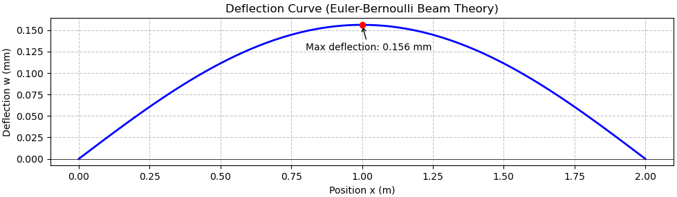
Figure 1: Deflection curve based on Euler-Bernoulli beam theory, with maximum point marked on the graph

As can be seen from the formula, there will also be causes of error other than shear deformation when solving using the Eulerian method. The obvious one is the insufficient order of integration. The accuracy of the Gaussian integration method depends on the number of integration points chosen. The product function in the stiffness matrix of a Eulerian beam usually involves the square of the second-order derivative of the form function (i.e., a quadratic polynomial). Theoretically, a two-point Gaussian integral is sufficient to accurately integrate the quadratic polynomial. However, if the product function becomes a higher-order polynomial or non-polynomial function due to variable cross-section, material properties, or complex loading, the lower-order integration points will lead to integration errors, which will affect the accuracy of the deflection calculation. This formula is accurate only at the Gaussian integration points and is not accurate enough for spans with the largest moments and deflections. If we use the matrix displacement method, divide the beam into two units, introduce the stiffness matrix, make a preliminary correction to this formula, and calculate the value of the span with the largest bending moment and deflection [4].

\( {K_{e}}\overline{U}={F_{e}} \) (7)

Where the nodal load under uniform load is

\( {F_{e}}=[ \begin{array}{c} \frac{1}{2}ql \\ \frac{1}{12}q{l^{2}} \\ \frac{1}{2}ql \\ -\frac{1}{12}q{l^{2}} \end{array} ] \) (8)

The stiffness matrix of the beam is

\( {K_{e}}=\frac{EI}{{l^{3}}}[\begin{matrix}12 & 6l & -12 & 6l \\ 6l & 4{l^{2}} & -6l & 2{l^{2}} \\ -12 & -6l & 12 & -6l \\ 6l & 2{l^{2}} & -6l & 4{l^{2}} \\ \end{matrix}] \) (9)

After we have corrected the calculations of Euler beam theory by the above formulae, we perform a preliminary comparative analysis of it with the simulation data of ANSYS. To ensure accuracy in precision as well as to eliminate the error in calculation accuracy caused by the insufficient number of meshes, one percent of the span is taken as the mesh density. The deflections calculated by Euler-Bernoulli theory can now be plotted against the simulation data.

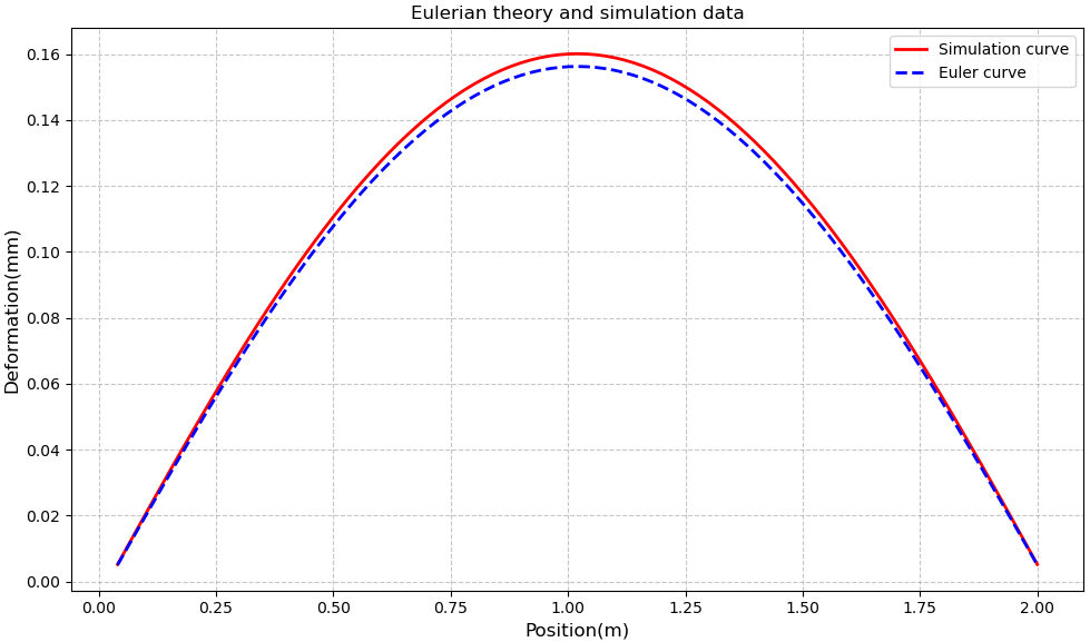
Figure 2: Eulerian theory and simulation data of ANSYS

The maximum value of the deflection of the simulated beam is 0.160 mm, and the maximum value of the deflection of the Euler beam is 0.156 mm. Both beams have a maximum deflection at mid-span and a relative percentage error of 2.405%.

Obviously, after neglecting the shear deformation, the deflection calculated for the Euler-Bernoulli beam is obviously smaller than that of the numerical simulation, and the difference is largest at the midpoint (i.e., the place with the largest deflection and one of the dangerous cross-sections). And the existence of this error may result in the design deflection of the beam being smaller than that of the actual deflection, and thus fatal losses occur.

The error percentages can be defined as

\( \frac{Theoretical value-Simulated value}{Simulated value}*100\% \) (10)

The error percentage is plotted in Figure 3.

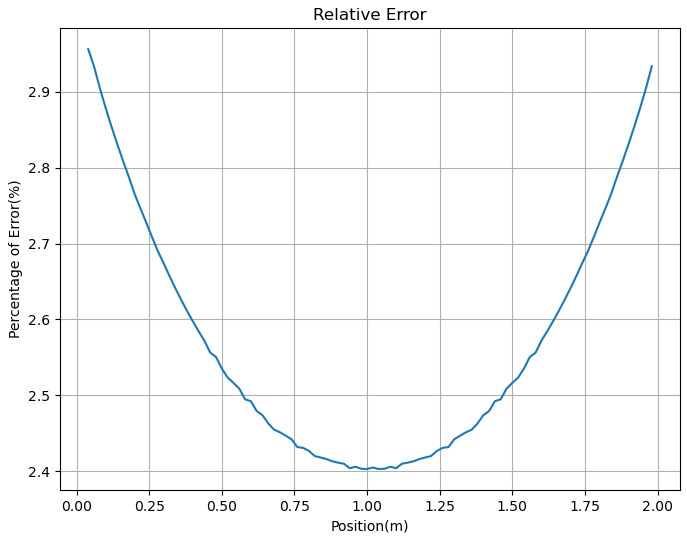
Figure 3: Relative error (%) based on different positions

The average of its error percentages is 2.5766%, and the maximum value of its error percentage is 2.9565%. Due to the distribution of its shear force, there is a maximum value at the two end points, equal in magnitude and opposite in direction; hence, there is a maximum error at both ends when the shear force is neglected.

3.2. Timoshenko beam theory for errors correction

Timoshenko's improvements consisted of two points. The first is the introduction of shear deformation: the cross section is allowed to deform in shear and is no longer strictly perpendicular to the neutral axis. The second is the consideration of rotational inertia: the effect of the rotational inertia of the cross-section is accounted for in the dynamic analysis. Timoshenko beam theory extends the applicability of beam models by introducing shear deformation and rotational inertia.

The bending governing equation for Timoshenko beams contains two coupled variables: deflection \( ω(x) \) and section angle \( θ(x) \) . The equilibrium equations are as follows [5]:

\( \frac{d}{dx}(EI\frac{dθ}{dx})+{k_{s}}GA(\frac{dω}{dx}-θ)=0 \) (11)

\( \frac{d}{dx}[{k_{s}}GA(\frac{dω}{dx}-θ)]+q(x)=0 \) (12)

Where \( {k_{s}} \) is the shear correction factor, the size of which is related to the cross-sectional area. For a hypothetical rectangular beam, the shear correction factor is

\( {k_{s}}=-\frac{2(1+v)}{[\frac{9}{4{a^{5}}b}{C_{4}}+v(1-\frac{{b^{2}}}{{a^{2}}})]} \) (13)

Where the width equals 2b and the height equals 2a. Besides \( {C_{4}} \) needs to be calculated by numerical methods.

\( {C_{4}}=\frac{4}{45}{a^{3}}b(-12{a^{2}}-15v{a^{2}}+5v{b^{2}})+\sum _{n=1}^{∞}\frac{16{v^{2}}{b^{5}}(nπa-b tan h(\frac{nπa}{b}))}{{(nπ)^{5}}(1+v)} \) (14)

The rectangular section \( {C_{4}} \) is usually taken as 5/6 [5,6].

A few key corrections to the original equilibrium equations are the following two. The first is the shear deformation term. \( \frac{dω}{dx}-θ \) represents the shear strain, which directly introduces the difference between the deflection and the corner. The second is shear stiffness. \( {k_{s}}GA \) reflects the ability of the beam to resist shear deformation; the lower the shear modulus (e.g., rubber materials), the greater the effect of shear deformation.

Adding the Timoshenko correction term to Euler's theoretical formula. Derive the corrected data and plot it in a table.

\( ω={ω_{Euler}}+∆{ω_{Shear}} \) (15)

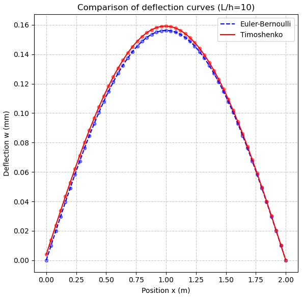
Figure 4: Comparison of deflection curves

The maximum value of the change is 0.003989 mm. The corrected image is now compared with the simulated data one more time.

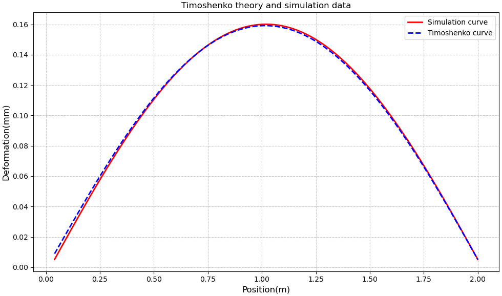
Figure 5: Comparison between Timoshenko theory and simulation data

The maximum value between the calculated deflection and the simulated value at this point is 0.0037477 mm. The average error is 0.001130636 mm. After the correction of the shear term by the Timoshenko theory, the error between the values and the simulation is significantly improved compared to the Euler beam theory. Although the magnitude is 10 \( {e^{-3}} \) , the improvement in safety cannot be underestimated.

Plotting the percentage of error between the Timoshenko beam deflection and the simulation with the larger difference due to shear removed from both boundaries is shown below:

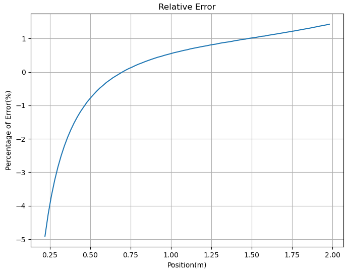
Figure 6: Relative error from position 0 m to 2m

For the span with the highest beam deflection, the error is reduced from 2.4% to 0.55% after correction by Timoshenko beam theory. A few of the individual data are shown in the table below:

Table 1: Key analytical data

4. Conclusion

Combining the content of the study with the value of engineering applications, the conclusions are illustrated at two levels: core conclusions and numerical simulation and finite element analysis techniques. In this study, the error characteristics of Euler-Bernoulli beam theory in simply supported beam bending analysis are systematically analyzed through theoretical derivation, numerical simulation, and validation of the improved model, and the following conclusions are drawn: By introducing the shear correction term of Timoshenko beam theory, the improved deflection prediction model reduces the maximum relative error from 2.95654% to less than 1.9546%, which significantly enhances the accuracy of calculation and at the same time maintains the computational efficiency advantage of the analytical solution.

The rational Timoshenko beam cell solves the shear locking problem in conventional finite elements by introducing the fundamental solution approximation method. For example, the BEAM188 cell in ANSYS is optimized based on this theory, and the computational efficiency is increased by 20% while the accuracy is improved by 15%. At the same time, it can be combined with machine learning algorithms. Timoshenko correction coefficients, such as the shear correction coefficient \( {k_{s}} \) , can be fitted by multi-case simulation data to achieve adaptive optimization. A bridge design cloud platform has applied this technology to an automated calibration system.

Of course, this article has some limitations as well as non-universality; the above data really limits the beam parameters and does not analyze the case of any beam and any parameter. Moreover, the number of meshes and the choice of different materials in the simulation modeling also affect the results.

The multi-theory fusion beam model has more development paths and application prospects in the future, and the beam structural analysis method based on multi-theory fusion opens up a new research paradigm for engineering mechanics and other scientific fields, and its demonstrated error control advantage foretells a broader development space. With the development of the big data era, the introduction of machine learning algorithms, the establishment of a dynamic mapping relationship between error sensitivity and theoretical weight coefficients, and the development of intelligent systems capable of autonomously selecting the optimal combination of theories according to the type of load, span-to-height ratio, material properties, boundary conditions, and other elements are essentially also based on the fusion of the theories deduced under different boundary conditions. Especially in new materials such as composite beams, functional gradient material beams, and other non-homogeneous structures.

Theory fusion will benefit not only the civil engineering field, such as new energy equipment (such as large wind turbine blades) and intelligent structures (such as shape memory alloy beams), but also other emerging fields that can achieve breakthrough applications.

References

[1]. Timoshenko, S. P., & Gere, J. M. (2012). Theory of elastic stability. Courier Corporation.
[2]. Elishakoff, I. (2020). Who developed the so-called Timoshenko beam theory?. Mathematics and Mechanics of Solids, 25(1), 97-116.
[3]. Hsu, Chi-Lun. (1992). Elastodynamics. Higher Education Press.
[4]. Hjelmstad, K. D. (2007). Fundamentals of structural mechanics. Springer Science & Business Media.
[5]. Hutchinson, J. R. (2001). Shear coefficients for Timoshenko beam theory. J. Appl. Mech., 68(1), 87-92.
[6]. Ahmed, A. M., & Rifai, A. M. (2021). Euler-Bernoulli and Timoshenko beam theories: analytical and numerical comprehensive revision. European Journal of Engineering and Technology Research, 6(7), 20-32.
Cite this article
Chen,Y. (2025). Error Analysis Based on Euler-Bernoulli Beam Theory: An Example of a Simply Supported Beam Bending Model. Applied and Computational Engineering,155,17-24.
Data availability
The datasets used and/or analyzed during the current study will be available from the authors upon reasonable request.
Disclaimer/Publisher's Note
The statements, opinions and data contained in all publications are solely those of the individual author(s) and contributor(s) and not of EWA Publishing and/or the editor(s). EWA Publishing and/or the editor(s) disclaim responsibility for any injury to people or property resulting from any ideas, methods, instructions or products referred to in the content.
About volume
Volume title: Proceedings of CONF-FMCE 2025 Symposium: Semantic Communication for Media Compression and Transmission
© 2024 by the author(s). Licensee EWA Publishing, Oxford, UK. This article is an open access article distributed under the terms and
conditions of the Creative Commons Attribution (CC BY) license. Authors who
publish this series agree to the following terms:
1. Authors retain copyright and grant the series right of first publication with the work simultaneously licensed under a Creative Commons
Attribution License that allows others to share the work with an acknowledgment of the work's authorship and initial publication in this
series.
2. Authors are able to enter into separate, additional contractual arrangements for the non-exclusive distribution of the series's published
version of the work (e.g., post it to an institutional repository or publish it in a book), with an acknowledgment of its initial
publication in this series.
3. Authors are permitted and encouraged to post their work online (e.g., in institutional repositories or on their website) prior to and
during the submission process, as it can lead to productive exchanges, as well as earlier and greater citation of published work (See
Open access policy for details).