1 Introduction

Air pollution is a problem of great concern for most countries, which has affected people's lives and health. Particulate matter (PM) plays an important role in air pollution and can cause various cardiovascular diseases, including heart failure, and increased mortality, and result in huge economic loss. A survey in 338 cities across 31 provinces of China in 2016 revealed that PM2.5-related premature mortality and morbidity caused economic loss as high as 101.39 billion US dollars, accounting for 0.91% of China's total GDP. The World Health Organization guidelines indicate that decreasing air pollutants (PM2.5, PM10, NO2, and O3) can reduce mortality by at least 0.5% per year because of decreased incidence of lung cancer, ischemic heart disease, stroke, and chronic obstructive pulmonary disease. Therefore, improved predictions of the concentration of PM2.5 and implementation of corresponding protective measures can effectively alleviate the health threat and economic loss caused by air pollution.

In recent years, many studies have applied deep learning models to improve the prediction accuracy of PM2.5 and overcome the problem of temporal correlation. The deep learning-based Transferred Bidirectional Long Short-term Memory (TL-BLSTM) model was proposed by Ma et al. to predict air quality. BLSTM models and transfer learning are superior to some conventional models such as Support Vector Regression (SVR) and Gradient Boosting Decision Tree (GBDT), especially for larger temporal resolutions. Mao et al. also used the neural network of the Long Short-term Memory Extension model (TS-LSTME) to predict the average PM2.5 in the Beijing-Tianjin-Hebei region in the next 24 hours. Some scholars have further improved the predictive power of PM2.5 by using high-resolution images with deep learning models. For example, Rijal et al. used images as data based on VGG-16, Inception-v3, and ResNet50 to predict PM2.5. The ordinal discrimination ability of the model at the last layer of the convolutional neural network model was improved by Zhang et al., who used the Rectified Linear Units as the activation function to alleviate the gradient disappearance problem and improve the stability of the model's air pollution prediction. Satellite imagery is now a critical data source to retrieve PM2.5 through the capability of revealing the scattering parameter of air pollutant. And various satellites can provide high-resolution and comprehensive observations, which can improve the predictions of surface PM2.5 concentrations. For example, satellite images have been successfully used to train a deep generative model to predict PM2.5 conditions in a 1536 km × 1280 km area. Using satellite sensor data from Modern Resolution Imaging Spectroradiometer (MODIS) also has great potential to enhance air quality monitoring at regional scales. The limitations of ground-based observations to monitor air quality have been shown for Texas, where NASA's MODIS has been used to monitor the migration of aerosol-borne pollutants across land and ocean surfaces with broader resolution. Another example comes from Zamani et al., who used PM2.5 data, meteorological features, and remote sensing Aerosol Optical Depth (AOD) data to train a random forest model and a Deep Neural Networks (DNN) model to predict the value of PM2.5 in Tehran City. Therefore, remote sensing satellite data play a vital role in the retrieval of PM2.5 concentrations.

While deep learning models are powerful, they are like black boxes. In other words, they are unable to provide information on which features play an important role in the prediction process. In contrast, some machine learning models, such as random forest, are able to deliver high accuracy outcomes with feature importance. Feature importance can facilitate access to interpretability and simplify the model, there by analysing which feature has more weight in the model. Random forest models are also less sensitive to missing values, which has been widely used for PM2.5 concentration predictions. Wang et al. calibrated the PM2.5 detector with a random forest model, which outperformed a linear model. A random forest algorithm was used for predicting the Air Quality Index of all uncovered areas in downtown Shenyang with an overall prediction accuracy of 81%, outperforming Naive Bayes, logistic regression, and single decision tree. AOD data, meteorological fields, and land-use features were used to train random forest models to estimate 24-hour daily ground PM2.5 concentrations in the United States. By using random forest models, it is possible to explore who can improve PM2.5 retrieval from satellite observations and meteorological conditions, and which features have a more prominent contribution to PM2.5 retrieval in meteorological conditions.

In this paper, we propose a set of experiments to reveal the importance of meteorological conditions from different vertical height data to PM2.5 retrieval. In addition, we explore data preprocessing methods to simplify the model while ensuring its stable performance. Finally, we determine which features are important and explore their connections further. Section 2 introduces data and the region of interest and explains the design of three experiments based on seven random forest models. Section 3 presents the comparison between the experimental results and random forest models. Finally, section 4 discusses the innovations and findings in this paper.

2 Data and methods

2.1 Data

We used a dataset from the Meteorological Science Knowledge Service System (http://k.data.cma.cn/mekb/?r=site/index), which covers 90 air quality monitoring stations in Sichuan Province, China, mostly distributed around Chengdu and Chongqing (Fig. 1). The monitoring stations recorded data every hour for a total of 60,000 samples from November 1, 2018, to November 30, 2018.

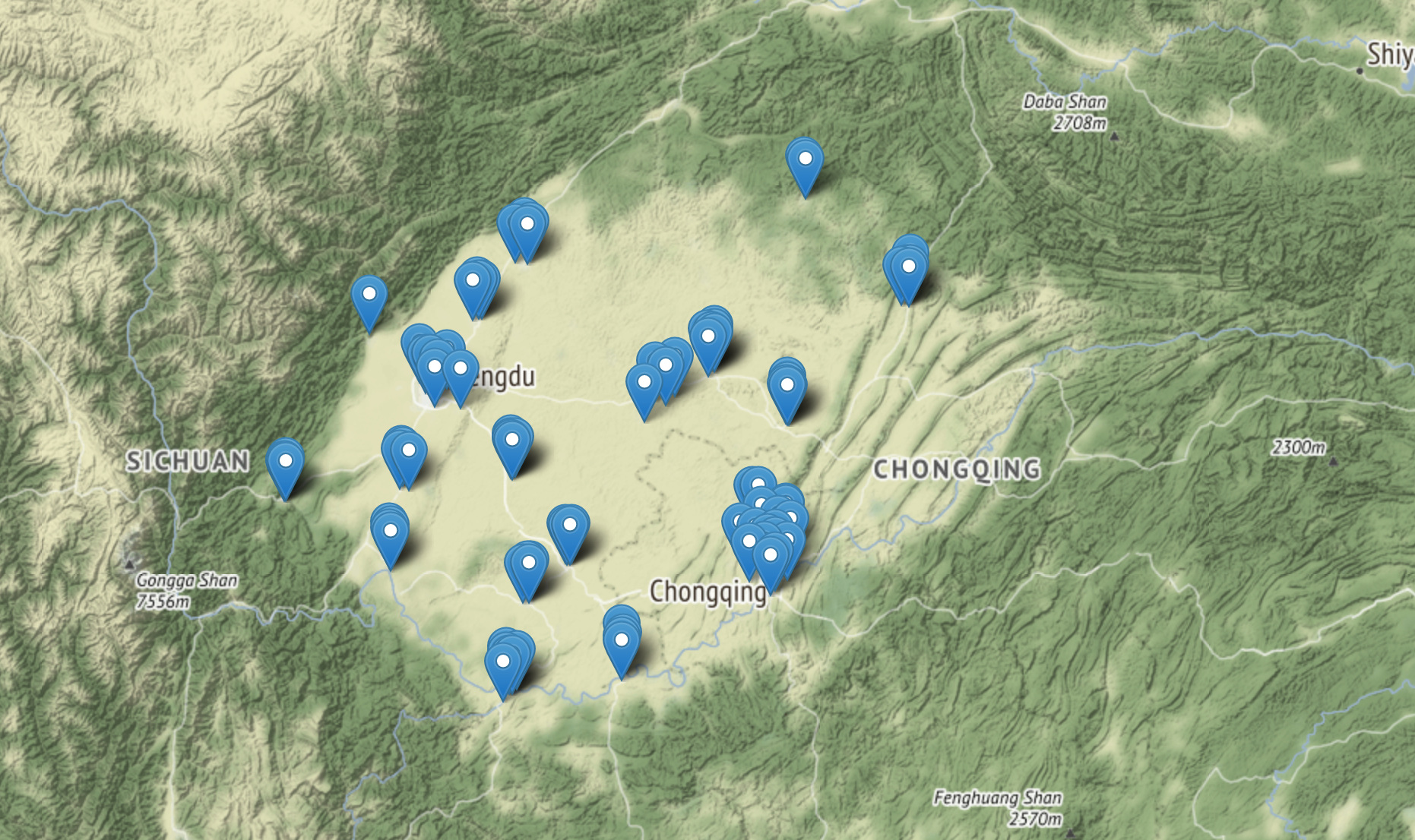
Figure 1. Location of air quality monitoring stations in Sichuan Basin, Southwest China. This dataset is composed of the ERA5 reanalysis dataset and FY-4A satellite data. ERA5 is a comprehensive set of reanalysis data from 1979 (soon going back to 1950) to near real-time, which incorporates as many upper-air and near-surface observations as possible. The ERA5 atmospheric model is combined with a land surface model and a wave model. In this paper, the ERA5 contains data of atmospheric pressure levels at 975hPa(near-surface) and 500hPa (indicating a mesoscale weather system) and uses the same features at two different atmospheric pressures, temperature, relative humidity, meridional wind speed, zonal wind speed, and vertical speed. The FY-4A satellite data are from China's second-generation geostationary meteorological satellite Fengyun-4 (FY-4A). The FY-4A satellite is equipped with a multi-channel scanning imaging radiometer, namely the Advanced Geostationary Radiation Imager (AGRI). AGRI has 14 channels and is able to acquire cloud images, aerosol information, and fire situations.

The concentration of PM2.5 varies diurnally. For example, the concentration of PM2.5 is relatively high in the morning and at night, while it decreases in the afternoon.

In addition, the concentration of PM2.5 on weekends is significantly lower than weekdays. One day was divided into three periods: morning (6 am-12 pm), afternoon (12 pm-19 pm), and night (19 pm-6 am). Then, the three time periods were added to the dataset as new features using the one-hot encoding technique. Similarly, the day of the week was determined based on the specific date of each day, and the new week feature was added to the data set.

Last, at the pressure levels of 975hPa surface and 500hPa mesoscale, the wind speed can be calculated by equation 1 and the wind direction can be calculated by equation 2 according to the wind speed (V) of the dimension and the wind speed (u) of the longitude in the dataset.

2.2 Experimental design

This paper designed three experiments to investigate the importance of different meteorological conditions for the retrieval of PM2.5. The first experiment, namely "EX1", included four parts. The first part used only satellite observations (EX1_sat); the second part was added extra meteorological conditions at 975hPa (EX1_sat_975hPa); the third part was added meteorological conditions at 500hPa (EX1_sat_500hPa); and the final part used all satellite observations and meteorological conditions at both 975hPa and 500hPa (EX1_all).

The second experiment, namely "EX2", included two parts. One part used only meteorological conditions at 975hPa (EX2_975hPa); and the other was added extra meteorological conditions at 500hPa (EX2_975hPa_500hPa).

The third experiment, namely "EX3", used a threshold to screen features. The optimal experiment, identified by comparing the performances of the six experiments in EX1 and EX2, was further simplified by setting an importance threshold.

2.3 Model evaluation method

To accurately assess the performance of random forest, three metrics were used to evaluate model performance, including the Root Means Square Error (RMSE), Mean Absolute Error (MAE), and the Coefficient of Determination (𝑅 2 ). Their equations are as follows:

where 𝑦 𝑖 * is the observed value, 𝑦 𝑖 is the retrieved value, and m is the number of samples in the dataset.

3 Results and Discussion

3.1 Adding Meteorological conditions improves the performance of PM2.5 retrieval

Tuning the parameters identified the optimal parameter for each experiment. Fig. 2 shows the scatter plots of the predictor and observations of the random forest model trained on four sets of input features in the first experiment (EX1).

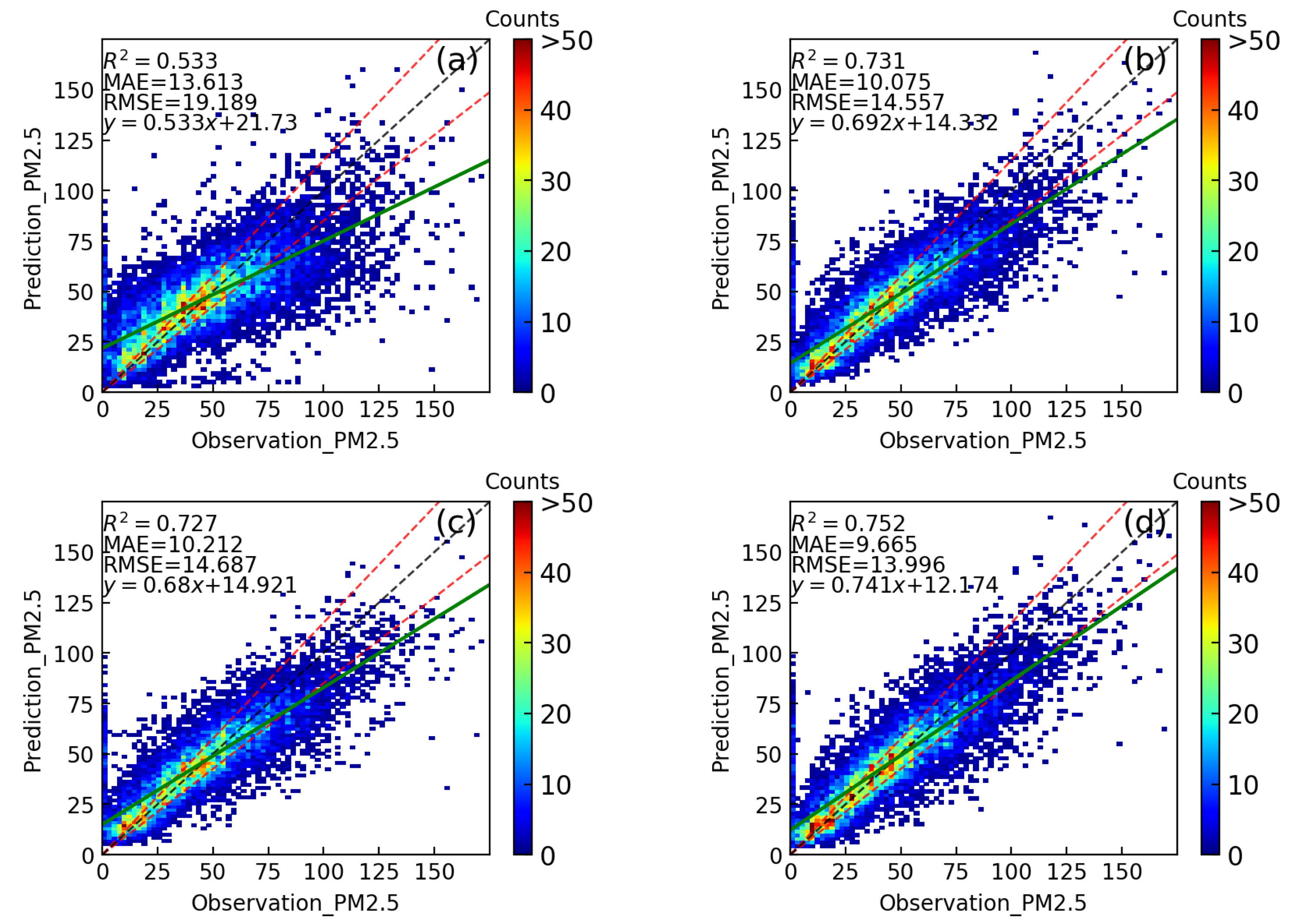
Figure 2. Scatter plots of EX1 results, comparison of observed (horizontal axis) and predicted (vertical axis) PM2.5 using the random forest model. (a) Using satellite observations only. (b) Adding meteorological conditions at 975hPa to satellite observations. (c) Adding meteorological conditions at 500hPa to satellite observations. (d) Adding meteorological conditions at both 975hPa and 500hPa to satellite observations. The black dashed line is the best fit line of the predicted results; the two green dashed lines are the 85% expected error envelope; and the green solid line is the fitted line of the experiment prediction result. The fitted line equation of the retrieval result (green dashed line) and the different colours of the scatter points represent the density of the data points, from sparse (in blue) to dense (in red).

As illustrated in Figure 2a, the random forest model for the retrieval of PM2.5 using only satellite data did not perform very well, with RMSE, MAE, and R2 being 19.188, 13.800, and 0.533, respectively. There is a huge gap between the fitted (solid green line) and the best fit lines (dotted black line). Additionally, the scattered points around both sides of the fitted line are not uniform. However, the scattered points of the bright areas in Fig. 2a are all concentrated around the best fit line.

In Figure 2b and Fig. 2c, meteorological conditions at 975hPa and 500hPa were added to satellite observations. With the added meteorological conditions, the fitted line of Fig. 2b and Fig. 2c is close to the expected error envelope, while RMSE, MAE, and R2 are better than for EX1_sat (Fig. 2a). Furthermore, according to the values of RMSE, MAE, and R2, the result of part 2 for EX1_sat_975hPa (Fig. 2b) is slightly better than part 3 for EX1_sat_500hPa (Fig. 2c), with differences of 0.13, 0.137, 0.004, respectively.

In Figure 2d, the meteorological conditions at 975hPa and 500hPa were added to the satellite observations, which resulted in the fitted line being closer to the expected error envelope compared with EX1_sat_975hPa (Fig. 2b) and EX1_sat_500hPa (Fig. 2c). The RMSE and MAE of EX1_all are 0.021 and 0.41 lower than for EX1_sat_975hPa, respectively, while the R2 is 0.021 higher.

In EX1, satellite observations alone did not perform well in PM2.5 retrieval, but the addition of meteorological conditions greatly improved the performance of the experiment. Combining satellite observations and meteorological conditions at both 975hPa and 500hPa provided the most accurate retrieval of PM2.5.

Feature importance plays a crucial role in predictive modeling projects, which provides insights into data, models, and how to reduce dimensionality and select features to improve the efficiency and effectiveness of predictive models.

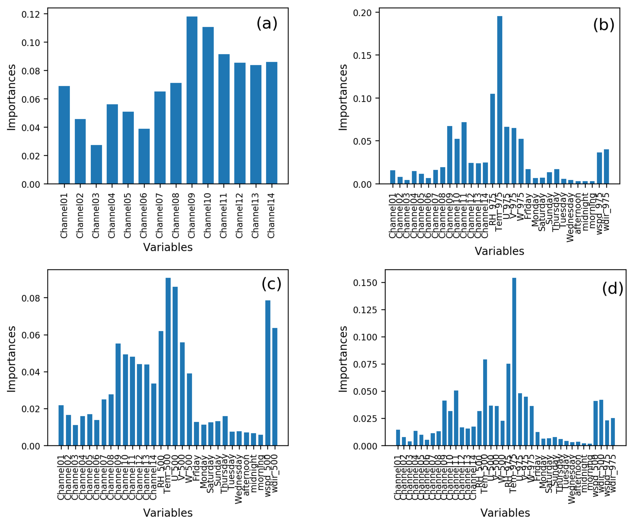
Figure 3. The importance of features in the four experiments in EX1. (a) Using only satellite observations. (b) Adding meteorological conditions at 975hPa to satellite observations. (c) Adding meteorological conditions at 500hPa to satellite observations. (d) Adding meteorological conditions at both 975hPa and 500hPa to satellite observations. The ordinate is the value of importance, and the abscissa is the feature name.

Figure 3a shows the feature importance when 14 channels of AGRI observation were used. Channels 9, 10, and 11 are more important than other channel features with the importance being more than 0.08. Channel 3 is the least important, which is about 0.02.

As illustrated in Fig. 3b and Fig. 3c, the importance of temperature is the highest. The importance of some features, such as time of the week and time of the day which are processed by the one-hot encoding, is below 0.02. Fig. 3b shows that the importance of temperature is higher than that of other features. For example, the factor is nearly 0.1 higher than that of relative humidity. Fig. 3c shows that, in addition to temperature, the features related to wind speed are also particularly important. The importance of vertical wind speed, in the second place, is about 0.08, and wind speed and wind direction after data preprocessing are ranked third and fourth, respectively.

EX1_all (Fig. 3d) used all satellite observation and meteorological conditions at both 975hPa and 500hPa. Fig. 3d shows the change in feature importance when atmospheric pressure 500hPa and 975hPa datasets based on satellite observation (EX1_sat) were used. The temperature at 975hPa is the most important, which is more stable and important than the temperature at 500hPa. Nevertheless, the temperature at 500hPa ranks second in importance, indicating that the temperature feature is the most important in the experiment. The wind speed and wind direction of the data processed by one-hot encoding also show a good performance, especially at 500hPa, compared with 975hPa. The importance of channel01-channel08 is about 0.02, which can be ignored. While the importance of channel09-channel14 is about 0.05. The importance of day of the week and time of day period features is weak, which is less than 0.02. From Fig. 3, it can be found that the temperature feature is significant in four experiments trained with different datasets. The importance of the processed new features wind speed and wind direction in the four experiments is quite satisfactory. However, the importance of day of the week and time of day period features remained below 0.2 in EX1_sat_975hPa (Fig. 3b), EX1_sat_500hPa (Fig. 3c), and EX1_all (Fig. 3d), indicating that their importance is relatively low.

3.2 PM2.5 Retrieval based on only Meteorological conditions

The second experiment (EX2) involved only meteorological conditions and contained two sets of input features. One set had only meteorological conditions at 975hPa (EX2_975hPa) as input while the other added extra meteorological conditions at 500hPa (EX2_975hPa_500hPa).

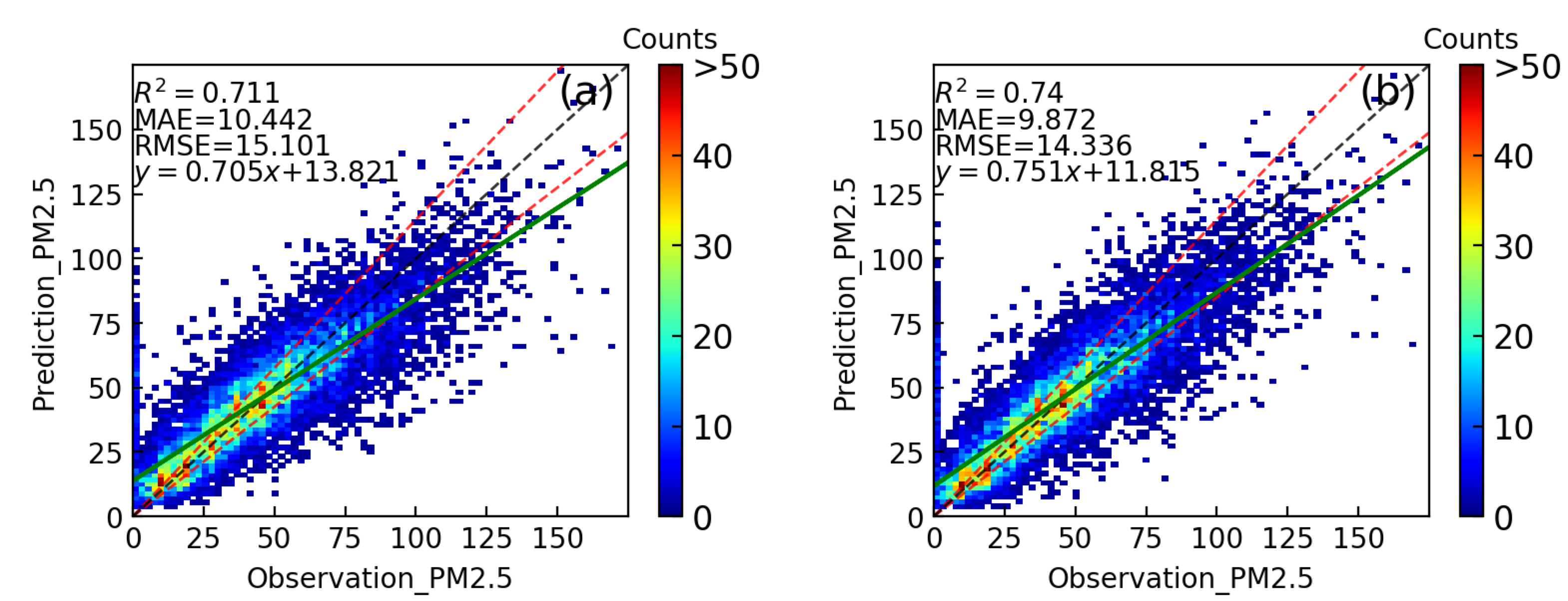
Figure 4. Scatter plots of the predicted and observed values of the two random forest models that only used meteorological conditions (EX_2). (a) Using only meteorological conditions at 975hPa. (b) Adding extra meteorological conditions at 500hPa. The ordinate is the predicted value, while the abscissa is the observed value. The black dashed line is the best fit line of the predicted results; the two green dashed lines are the 85% expected error envelope; and the green solid line is the fitted line of the experiment prediction result. The different colors of the scatter points represent the density of the data points, from sparse in blue to dense in red.

The experiment trained using meteorological conditions at 975hPa (Fig. 3a) did not perform as well as that adding extra meteorological conditions at 975hPa (Fig. 3b). The RMSE and MAE of EX1_975hPa_500hPa decreased by 5.06% and 5.45%, respectively, compared with EX2_975hPa; and the 𝑅 2 increased by 4.08%. In addition, the angle between the scatter fitting line (green solid line) and the best fitting line (black dotted line) of EX1_975hPa_500hPa is smaller than that of EX2_975hP (Figure 4).

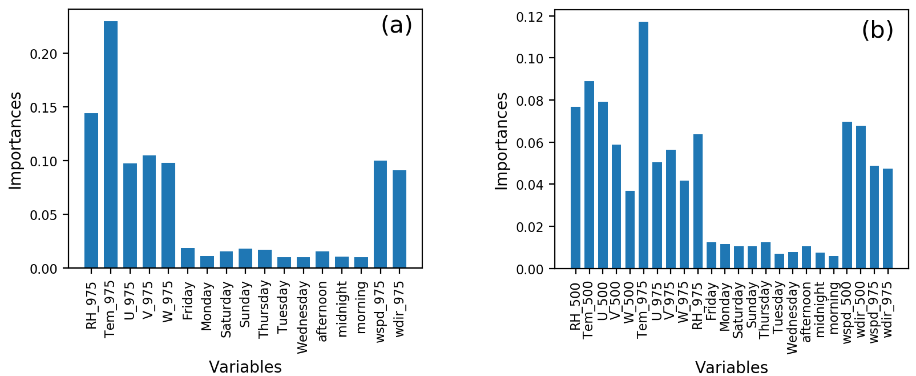
Figure 5. Importance of features in the two EX2 experiments. (a) Using only meteorological conditions at 975hPa. (b) Adding extra meteorological conditions at 500hPa based on EX_975hPa (a). The ordinate is the importance value and the abscissa is the feature name.

As illustrated in Fig. 5a, the temperature has the highest importance of more than 0.2, followed by relative humidity at around 0.14. The importance of the features related to wind speed and wind direction is about 0.09. However, the importance of the new features of week and date processed by the one-hot encoding is not very prominent, which is basically maintained at around 0.02.

As illustrated in Fig. 3b, the temperature at 975hPa is the most important, which is more stable and important than the temperature at 500hPa. Nevertheless, the temperature at 500hPa ranks second in importance, indicating that the temperature feature is the most important in the experiment. The wind speed and wind direction of the data processed by one-hot encoding also show a good performance.

Especially, when the pressure level is 500hPa, the importance of wind speed and wind direction ranks fifth and sixth respectively. The importance of day of the week and time of day is also weak like for EX2_975hPa, being less than 0.02.

In EX1 and EX2, the random forest model that used all satellite observation and meteorological conditions at both 975hPa and 500hPa datasets (EX1_all) performed best, followed by the one trained using meteorological conditions at both 975hPa and 500hPa (EX2_975hPa_500hPa). In contrast, random forest using only satellite observations (EX1_sat) performed the worst. The importance of temperature is the most prominent among the dataset features, especially the temperature at 975hPa.

3.3 Feature importance based feature selection

In EX1_all, the temperature feature is particularly prominent. Especially, the temperature at pressure level 975hPa is the most important, which is about 0.15 and far more than other features. The importance of satellite observations is not obvisouly high, being around 0.025. The EX1_all performed the best among all experiments and covered satellite observation and meteorological conditions at both 975hPa and 500hPa datasets. Therefore, only this experiment explored whether there was a significant change in the performance of the experiment after setting the importance threshold. The feature importance threshold in EX1_all was set to 0.04, and the sum of the feature importance selected according to the threshold was 0.58. The features selected and their corresponding importance are shown in the following table:

Table 1. Features selected according to the threshold.

Parameter name

Feature importance Satellite observations channel11 0.054 channel09 0.041 Meteorological conditions Temperature at 975hPa 0.154 Temperature at 500hPa 0.079 relative humidity at 975hPa 0.075 wind speed v-component 0.048 wind speed u-component 0.045 wind direction 0.042 wind speed 0.040 Table 2. Experiment performance metrics. RMSE MAE 𝑅 2 EX1_all a 13.996 9.665 0.752 EX3 b 14.682 10.250 0.726 a Original experiment results. b Experiment results using features selected with an importance threshold of 0.04.

The model's performance with the threshold set in EX1_all and the model without the threshold set before was basically similar, with RMSE, MAE, and R2 differences of 0.686, 0.585, and 0.026, respectively. Although EX1_all and EX_3 have similar retrieval capability, the number of features was reduced from 38 to 9, indicating that the experiment complexity was greatly simplified while retaining its retrieval power.

4 Conclusion

This paper explored the importance of meteorological conditions in PM2.5 retrieval performance, which is innovative in terms of combining meteorological data, such as wind speed, temperature, and relative humidity, with channel data outputs from satellite images. The retrieval ability of the input data was explored through a series of experiments. In the first experiment, satellite observations and meteorological conditions were used to explore whether satellite observations could improve PM2.5 retrieval capabilities. The second experiment only used meteorological conditions to explore the PM2.5 relative retrieval performance of meteorological conditions and satellite observations. Finally, through the importance analysis of the features in the experiments, we explored whether satellite image data could improve the model's predictive performance compared with the meteorological condition. There are four major conclusions as follows:

1) PM2.5 retrieval becomes more accurate after adding meteorological conditions to satellite observations, which performs even better when adding meteorological conditions at 500hPa and 975hPa. That indicates the addition of meteorological data can improve the retrieval performance of ground PM2.5 retrieval. Another finding is the results adding conditions at 975hPa are better than 500hPa, 2) When adding meteorological conditions (at 500hPa and 975hPa) to satellite observations, the accuracy of PM2.5 is best, and the condition of 975hPa is better than the condition of 500hPa. This also indicates that although mesoscale meteorological conditions (at 500hPa) are not closely related to near-surface PM2.5, they improve model accuracy. The present study also reveals that PM2.5 is not only affected by near-surface weather conditions but also related to meso-scale weather systems.

3) Using meteorological conditions to retrieve PM2.5 seems promising, which indicates that PM2.5 is dominated by weather factors rather than the real-time characteristics of atmospheric pollutants provided by observational data. Whether using meteorological conditions of 975hPa or both 975hPa and 500hPa, PM2.5 retrieval is superior to satellite observations, and R^2 increased by 0.178 and 0.207, respectively. The importance of 500hPa and 975hPa temperatures is the highest, indicating that static atmospheric conditions have an important impact on ground PM2.5.

4) Using a threshold of feature importance to screen features shows that the PM2.5 retrieval accuracy changes little, indicating that the input features can be simplified and the training time can be shortened by selecting key features.

In the future, we will work on improving PM2.5 retrieval using satellite data considering their advantages of high resolution and low cost. We will explore the use of data engineering techniques to enhance PM2.5 retrieval combined with deep learning frameworks and satellite data.Shah A S, Langrish J P, Nair H, McAllister D A, Hunter A L, Donaldson K, . . . Mills,N.L. (2013).

Ensemble of Deep Neural Networks

for estimating particulate matter from images. 2018 IEEE 3rd International Conference on Image, Vision and Computing (ICIVC). doi:10.1109/icivc.2018.8492790Zhang C, Yan J, Li C, Rui X, Liu L, & Bie R. (2016). On estimating air pollution from photos using convolutional neural network. Proceedings of the 24th ACM International Conference on Multimedia. doi:10.1145/2964284.2967230Ravuri S, Lenc K, Willson M. et al. (2021) Skilful precipitation nowcasting using deep generative models of radar. Nature 597, 672-677. https://doi.org/10.1038/s41586-021-03854-zHutchison K D. (2003). Applications of MODIS satellite data and products for monitoring air quality in the state of Texas. Atmospheric Environment, 37(17), 2403-2412. doi:10.1016/s1352-2310(03)00128-6Zamani Joharestani M, Cao C, Ni X, Bashir B, & Talebiesfandarani S. (2019). PM2.5 prediction based on Random Forest, XGBoost, and deep learning using Multisource Remote Sensing Data. Atmosphere, 10(7), 373. doi:10.3390/atmos10070373Wang Y, Du Y, Wang J, & Li T. (2019). Calibration of a low-cost PM2.5 monitor using a random forest model. Environment International, 133, 105161. doi:10.1016/j.envint.2019.105161Hu X, Belle J H, Meng X, Wildani A, Waller, L. A., Strickland, M. J., & Liu, Y. (2017).

Estimating PM2.5 concentrations in the conterminous United States using the Random Forest Approach. Environmental Science & Technology, 51(12), 6936-6944.

doi:10.1021/acs.est.7b01210Yu R, Yang Y, Yang L, Han G, & Move O. (2016). Raq-a random forest approach for predicting air quality in urban sensing systems. Sensors, 16(1), 86. doi:10.3390/s16010086Watson J G, & Chow J C. (2002). A wintertime PM2.5 episode at the Fresno, CA, supersite. Atmospheric Environment,36(3), 465-475. doi:10.1016/s1352-2310(01)00309-0Tong R, Liu J, Wang W, & Fang Y. (2020). Health effects of PM2.5 emissions from on-road vehicles during weekdays and weekends in Beijing, China. Atmospheric Environment, 223, 117258. doi:10.1016/j.atmosenv.2019.117258