1. Introduction

1.1. Psychological background of MBTI

MBTI (Myers-Briggs Type Indicator) is a theoretical model of personality types that gives a judgment and analysis of a person's personality. It is a theoretical model that mainly reports how people perceive the world and their psychological preferences when making decisions. MBTI model concludes four dimensions: attitude, dominant information-gathering function, dominant decision-making function, and perceiving or judging function, from people's complex personalities [1]. Each dimension includes two opposite categories: Extroversion/ Introversion, Sensing/ Intuition, Thinking/ Feeling, Judging/ Perceiving [2]. People produced 16 unique qualities by choosing preferred qualities in each category, and the results are composed of four-dimensional initials, such as ISFJ and ENTP, as shown in Table 1.

Table 1. 16 unique qualities with four-dimensional initials divided into two opposite categories.

In today's society, MBTI is widely used in various industries worldwide due to its simple operation, mature theoretical framework, low cost, and noticeable effect. The testing results effectively explain people's behavioral differences, and they provide individuals with a better understanding of each other.

For example, MBTI test results can be applied to personal training, team building, career development planning, recruitment, and selection of medical personnel. It was found that the personality type of ESTJ dominated the test results of medical staff[3]. The finding shows that career choice does correlate with a person’s personality type.

1.2. Background of personality type prediction using computer technology

In recent years, the rapid development of natural language processing technology and its mature technology in the field of text classification makes using computer technology to predict personality types become feasible. Researchers found that computer technology was as good as other methods in studying the problem, and it is even better than traditional methods in many scenarios.

In recent years, machine learning and deep learning technologies have improved tremendously, and their development has promoted the great progress of natural language processing technology. Many researchers have successfully used classical machine learning techniques and neural networks to predict MBTI personality types. Golbeck et al. conducted one of the first studies in 2011 using machine learning techniques for personality prediction and using regression analysis to analyze the number of friends and social network density of Twitter data [4].

Cui and Qi compared a variety of traditional machine learning methods in their recent study and finally found that SVM achieved relatively good results [5]. Zi et al. used the variant of CNN to study the short video data of users, and the method of personality classification prediction by using video data entered the research field of vision [6]. Pascale Fung et al. even used RNN as the basic technology to implement a language interactive system that can empathize according to the personality type of the interlocutor, Zara the Supergirl [7]. Hernandez and Knight made a good summary by comparing the effectiveness of multiple recursive neural networks in predicting MBTI personality type problems [8]. Furthermore, Sedrick and Cheng investigated the possible use of a fine-tuned BERT model in the generation of personality-specific languages [9].

1.3. Introduction to decision tree

Decision trees, as an essential method in the machine learning field, have been widely used around the world. Based on knowing all kinds of possibilities, it is a decision analysis method to obtain the probability that the expected net present value is greater than or equal to zero, evaluate the project risk, and judge its feasibility by forming a tree-like structure. There are two main types for decision trees to play a role in the data mining field: the classification tree and the regression tree. However, there could be more kinds with the ensemble method, like boosted trees, bootstrap aggregates (random forest), and rotation forest[10]. Decision tree is the simplest machine learning algorithm. It is easy to implement and visualize, also can be interpreted, completely in line with human intuitive thinking. Thus, this algorithm has become a great candidate for being applied to the classification mission of this MBTI dataset. The analysis of this dataset shows the lengths of the samples are quite limited. These samples can be easily transformed into vectors with limited attributes. This provides an ideal condition for using Decision tree Classification Algorithm. In addition, training a model with Decision tree Classification Algorithm usually requires less cost of time than that with Neural Network Algorithms. A model with high accuracy can be obtained within a few moments by using Decision trees. This efficient algorithm is definitely a temptation for machine learning users.

2. Primary method - decision tree

2.1. TF-IDF

Here, TF-IDF is chosen to vectorize the text data. TF-IDF is short for “Term Frequency – Inverse Document Frequency”. This method has been widely used in natural language processing. The formulas are given by Eq.(1) and Eq.(2) :

\( TF-IDF(t,d)=tf(t,d)*idf(t) \) (1)

\( idf(t) = log(\frac{1+n}{1+df(t)})+1 \) (2)

\( tf(t,d) \) is the frequency of term t in document d. \( idf(t,d) \) ， “inverse document frequency” ， represents the total number of documents? \( n \) is the number of documents. \( df(t) \) is the number of documents that contain the term t. After the computation, the resulting vectors will be normalized by the Euclidean norm [11]. The term with a higher TF-IDF value in the vectors will be attached with more importance and attention in future analysis.

2.2. Decision tree

The approach of decision tree predicting is quite simple. Resembling the trees in Data Structure, a decision tree consists of several nodes and leaves. Each node in the decision tree contains a simple classifier that can classify the current sample by comparing the most significant feature of the current sample vector with the threshold. Then, according to the classification result, the sample will go to the sub-branch for a more precise prediction via being further classified. After recursive partition in tree-formed classifiers, the sample comes to a leaf with an outcome of the final prediction.

Indeed, there are several modified algorithms of decision tree, and this work chooses one of the most popular models, CART. An example of CART is shown below.

There is a training set. The training set is given by Eq. (3) and the target vector is given by Eq.(4):

\( X=[\begin{matrix}0 & 0 & 0 \\ 1 & 1 & 1 \\ 0 & 1 & 0 \\ 1 & 0 & 1 \\ \end{matrix}] \) (3)

\( Y=[\begin{matrix}0 \\ 0 \\ 1 \\ 1 \\ \end{matrix}] \) (4)

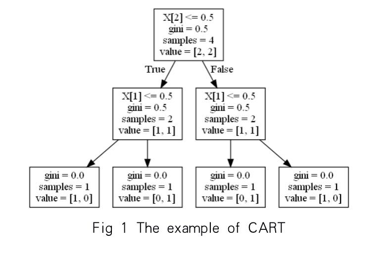
Figure 1. The structure of a decision tree trained with the training set given by Eq.(3) and Eq.(4).

The CART model trained with this simple training set is shown in Figure 1. In each block, the first row shows the condition of splitting (e.g. X[2] <=0.5). If the sample meets the condition, then it will go to the left branch, and vice versa. The second row shows the current Gini Impurity. In this algorithm, Gini Impurity is used to find the best split for this CART model. Gini impurity will be introduced later. The third row (samples) shows the number of samples split into the current node. The fourth row (value) shows the number of samples in each label.

2.3. Gini Impurity

Gini Impurity measures the accuracy of classification. The following formula shows the principle of Gini Impurity.

\( Gini Impurity=1-\sum _{i+1}^{n}{p_{i}}*(1-{p_{i}}) \) (5)

In this formula, \( {p_{i}} \) is the proportion of samples labeled with Label \( i \) in this node. When Gini Impurity is closer to zero, it implies a better performance of the current classifier. Thus, what needs to be done is to minimize the Gini Impurity. In CART, each classification node has two son nodes. In order to measure the performance of this classifier, Gini Impurity for both son nodes need to be computed. Then, multiply the proportion of samples in each son node with the corresponding Gini index and sum them up. In this way, the current classifier will be assessed.

The way to optimize each classification node is to minimize its Gini Impurity. The method for minimization is to traverse the rest of the possible attributes to find the best one as the condition for splitting, which is quite simple. After recursive computation, a well-trained model will be obtained.

3. Experiment

3.1. Dataset introduction & data visualization

The dataset used in the experiment comes from Kaggle, a huge online repository of community collected data and code. This dataset is one of the most widely used datasets about MBTI on Kaggle. It contains 8675 rows of data, which are classified into 16 categories: INFP, INFJ, INTP, INTJ, ENTP, ENFP, ISTP, ISFP, ENTJ, ISTJ, ENFJ, ISFJ, ESTP, ESFP, ESFJ, and ESTJ. Among these 16 categories, INFP and INFJ are the largest, with 21.2% and 17% respectively as shown in Figure 2.

For visualization of the dataset, seaborn and matplotlib were used to calculate and illustrate the distribution of all personality types. Figure 2 shows the proportion of all the personality types in the dataset using a donut chart. In this experiment, 60% of the data was used as a training set with a total of 5205 rows of data, and the remaining 40% of data was used as a test set to detect the accuracy of the model with a total of 3470 rows of data. In order to improve the accuracy of system prediction, the post was pre-processed before applying each model, which will be explained in detail in section 3.2. All posts used in the experiments were washed and non-text messages (including the linking parts) appearing in the post were cleared. After that, each post was separated into words.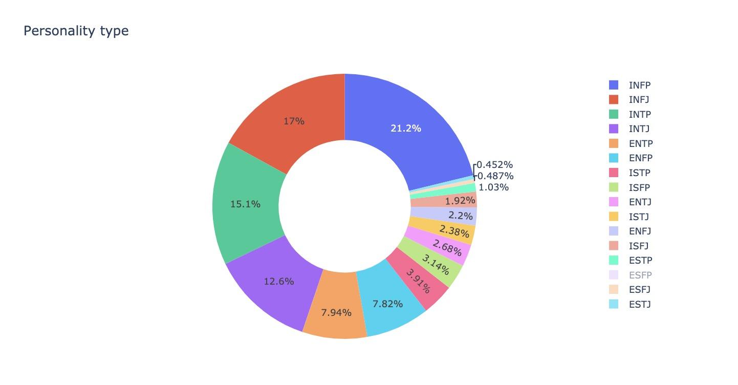

Figure 2. Percentage of occurrences for each personality type in the dataset.

3.2. Data preprocessing

Since the dataset was collected from the internet and contained a lot of posts, it is necessary to do the preprocessing and remove meaningless phrases. The data preprocessing is based on 4 major steps. First of all, remove the URL links because the dataset includes posts with comments, links, and punctuation marks. Then, count the number of words of every post after removing invaluable information and encoding the labels. Since the English letters cannot be recognized by the computer, giving them a default value is necessary, so then the computer knows what this letter corresponds to (e.g. giving the same personality type the same type of encoding, assigning INFJ as 8 and separating those personality types into 4 categories where each includes 2 letters, and giving each of the letters a label that is either 1 or 0). After that, Vectorize the previous steps by using Term Frequency Inverse Document Frequency, which is called TF-IDF for vectoring [12]. An inverse weighting is introduced here to scale down the words that occur too frequently. By calculating term frequency values and inversing the document frequency, redundant words will not play such a big part in differentiating between the documents. After that, multiplying and normalizing 2 matrices and their product will turn the result into a TF-IDF matrix, making it much easier for computers to identify. The final step is splitting the dataset into a training set for 60% and a testing set for 40%.

The following Figure 3 shows the concrete steps for data preprocessing in this dataset.

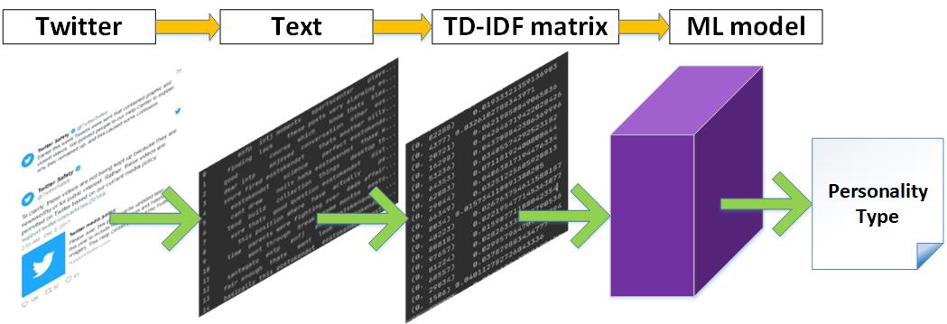
Figure 3. Steps for data preprocessing.

3.3. Major method experiment

The algorithm being used in the work is a decision tree. First, the words in the text were converted into a word frequency matrix. The term frequency (TF), the number of times each word appears in the post, and the inverse document frequency (IDF) of each word was then counted. If a word is very common, its IDF will be smaller. In the next step, the work arranged the product of TF and IDF from largest to smallest with the keywords of the post at the top. This is because the word not only appears frequently in posts, but it is also an uncommon word in the corpus. According to the keywords of posts under different labels, this work extracted features of these labels. In the project, there is a setting label for each category of these features to ensure that non-numerical features can be mapped to numerical values. Then, these attributes are input into the decision tree and classified each attribute from the root node. After the training of the decision tree model, it appears that the accuracy of the training set can reach 0.83, and the accuracy of the test set can reach 0.51.

Decision trees are being used in the process of binary classification of each attribute to finally get the MBTI type that corresponds specifically to each post. In the data preprocessing stage, the attributes have been listed from large to small. In the model, 107 attributes are used for the experiment with a depth of 7 . Therefore, the system will get the MBTI results of POST based on two classifications of 107 attributes. Since the accuracy of work is not particularly high, Gini indexes are used to detect the suitability of each attribute. The more impure the attribute is, the larger the Gini index value is. For example, if there is only one category for all the data in the training set under the attribute, the Gini index is 0. If the number of two categories is the same, it is 1 / 2. At this stage, the smaller the Gini index value, the more successful the classification is. However, in this experiment, it can be noticed that more than 60% of the attributes have a Gini value over 0.5. This indicates that the attributes selected for this experiment were not very successful. This is one of the major reasons why the accuracy of this model is only 0.51.

Due to the unequal number of data below 16 classifications in the dataset, which has a significant impact on the accuracy of the model prediction, adding a column of MBTI feature pairs as (I vs E; N vs S; F vs T; P vs J) to train each feature independently during the experiment would greatly reduce the impact of the dataset imbalance. So to further improve the accuracy of the model, a separate decision tree is used for each set of features in the experiments.

The following four figures show the accuracy of the model when the attributes are 200, 1000, 2000, and 3000 respectively for different depths. The comparison shows that the accuracy of the model when attributes are 3000 is not as high as when attributes are 200, 1000, and 2000. It is possible that the model is overfitted when too many attributes are used in the experiment. By comparing the accuracy of different depths in Figure 4, Figure 5, Figure 6 and Figure 7, the accuracy of the model is highest when the depth is 10. Therefore, the final accuracy is 0.73862 for I/E classification, 0.84179 for N/S classification, 0.59539 for F/T classification, and 0.61095 for J/P classification. It can be found that they are all much greater than 0.51.

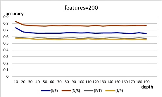
Figure 4. Accuracy when features are 200.

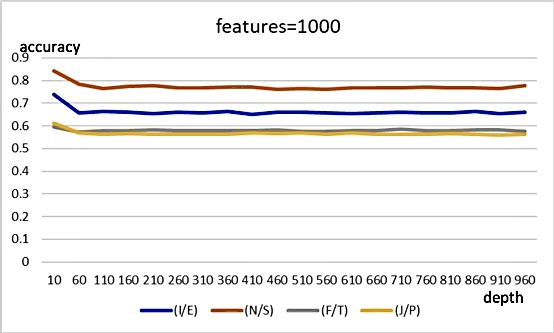
Figure 5. Accuracy when features are 1000.

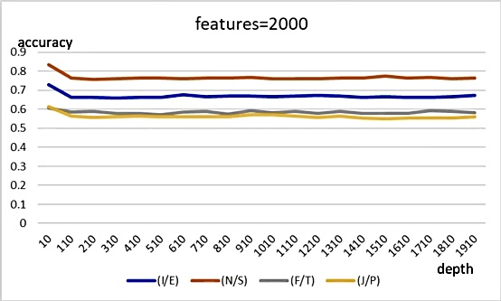
Figure 6. Accuracy when features are 2000.

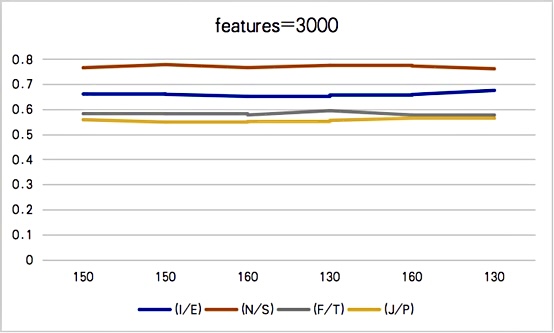
Figure 7. Accuracy when features are 3000.

In Figure 8, there are four normalized confusion matrices that show the contrast between the prediction results and real labels from the test set. In each chart, blocks with coordinates [0,0] and [1,1] refer to correct prediction while other blocks refer to the wrong prediction. The decimal number in each block shows the proportion of samples in the totality with the same true label. In addition, the sum of decimals in each row equals one.

Unfortunately, it’s obvious that some of the samples have been misclassified. In the classification of first and second labels, over half of the samples with tab “1” have been misclassified. This is probably caused by the unbalanced training set, which leads to the limitation of prediction accuracy. However, using four classifiers to classify four aspects of samples has improved the accuracy of the model, better than using one classifier to classify the combination of four aspects at one time.

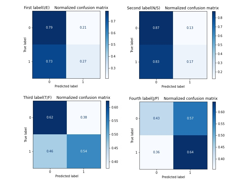
Figure 8. Confusion matrices for four different labels in decision tree method.

3.3.1. XGBoost. XGBoost[13] is an optimized distributed gradient enhancement library designed to be efficient, flexible, and portable. It implements machine-learning algorithms in the Gradient Boosting framework that can solve many data science problems quickly and accurately.

After putting the dataset in, XGBoost goes through multiple rounds of iteration, each of which generates a weak classifier, and each classifier is trained based on the residual of the previous round. The requirements for weak classifiers are generally simple enough and have low variance and high bias. The process of training is to continuously improve the accuracy of the final classifier by reducing the deviation.

XGBoost shows stability and relatively good performance in MBTI classification. Table 3 shows that XGBoost is more stable than other methods in the classification of four different letters, especially in the first two letters.

As shown in Figure 9, XGBoost shows a great performance in identifying true positives (0.78) and true negatives (0.6), but it shows a mediocre performance in finding false positive (0.4).

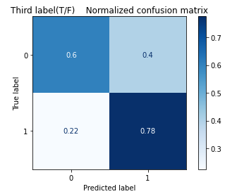
Figure 9. Confusion matrix for the third label (T/F) in XGBoost.

The original accuracy for XGBoost is 0.58, the highest accuracy among all models, as shown in Table 2. When using the modified method to run four pairs separately, Table 3 shows that the accuracies for all these pairs have bumped up: the First(I/E), the Second(N/S), the Third(T/F), and the Fourth(J/P) Labels become 0.7639, 0.8592, 0.6993, and 0.6186, where the first and second labels increase most significantly.

3.3.2. Random forest. Random forest is an algorithm that integrates multiple trees through the idea of ensemble learning. Its basic unit is decision trees. Each decision tree is a classifier, for each input sample, N trees will have N classification results. Random forest, on the other hand, integrates all the classification voting results and designates the category with the most votes as the final output, which embodies the Bagging guiding philosophy.

For the dataset in this experiment, different decision tree estimators randomly choose equal-amount samples in the whole dataset as their own training set. After training, each estimator will give their own classification of the samples, and the result label, which has the greatest amount, will be stated as the final result of the random forest.

Random forest is just like XGBoost, shown in section 3.5, demonstrating that it is more stable and achieved better results in the first two letters.

Compared to other methods, random forest has the best performance in identifying the true positives (0.82), but it shows a poor performance in finding the true negatives (0.55) and false negatives (0.45), shown in Figure 10.

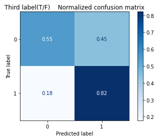
Figure 10. Confusion matrix for the third label (T/F) in random forest.

Overall, Table 2 demonstrates that random forest achieves an accuracy of ​​0.5659, the second-highest accuracy in all models. After separating into four pairs, this model gives much better accuracy for each one of the pairs. The accuracies for each one of the pairs is listed as First Label (I/E) 0.7779, Second Label (N/S) 0.8606, Third Label (T/F) 0.7021, and Fourth Label (J/P) 0.6301, in which the second label accuracy has improved the most, as shown in Table 3.

3.4. Control experiment

The method used in this experiment is also compared with other former methods used in MBTI classifications, such as the bidirectional LSTM, to validate the quality of classification results. The training and test data are randomly chosen in the whole data set, where 60% of the dataset is for training and the rest is for testing. The epoch is set to 500 for each method.

3.4.1. 1D CNN. Convolutional Neural Networks (CNNs) are a class of biologically inspired neural networks. It has been widely used in image recognition, natural language processing, speech recognition, etc.In a One-dimensional Convolutional Neural Network (1D-CNN), the data will be entered into the network after preprocessing. Depending on different model parameters, people can control the amount of data input. This experiment used ReLU and softmax to activate only parts of the neurons at a time. Max Pooling, a type of pooling/subsampling, was then used to extract the most representative features, which effectively reduces the output scale, and thus reduces the number of parameters needed by the model. Finally, the fully connected layer maps the multidimensional features into a one-dimensional output[14].

Table 2 shows that the original accuracy gained for 1D-CNN is 0.25, which is one of the lowest accuracies over all other models used in the control experiment. After running each feature pair of MBTI in 1D-CNN, the accuracies for the First(I/E) and Second(N/S) Labels lowered to 0.2285 and 0.1447, while the accuracies for the Third(T/F) and Fourth(J/P) Labels soared to 0.5343 and 0.6061, respectively, as shown in Table 3.

3.4.2. Bidirectional long short-term memory (Bidirectional LSTM). Long Short-Term Memory(LSTM) is a novel recurrent network with an appropriate amount of gradient-based learning algorithm[15]. It understands the context behind input and bridges distant time intervals even under noisy, incompressible input sequences, without loss of its short-term memories.

After inputting the dataset, LSTM splits the input data into time sequences. The forget gate determines whether to keep or throw away information from the cell state. The input gate and a tanh layer then decide the values needed to be updated and what the new values are. Finally, the cell state will go through tanh layer and only output the information needed for the experiment.

Bidirectional LSTM is an evolutional model from LSTM, where it duplicates the first recurrent layer and reverses the copy to be the second. With the two layers, the patterns could be gained from running through in the positive direction or in the negative direction.

The original accuracy for Bidirectional LSTM from the experiment is 0.20, which is one of the lowest results compared with the ones from other models, as shown in Table 2. When four pairs of labels are separated, shown in Table 3, the accuracy for the Second Label (N/S) lowered to 0.1398, while the First(I/E), Third(T/F), and Fourth(J/P) Labels rises to 0.2207, 0.5409, and 0.5965, respectively. Among these labels, the first and second labels have not changed much.

3.4.3. Linear regression. Linear Regression is a linear method that models the relationship between scalar responses and one or more explanatory variables. It is simple to calculate, easy to understand and present, and suitable for both numerical and nominal data. Basically, linear regression was developed in the statistical field and it was always used by researchers to understand the relationship between input and output numerical variables.

Linear Regression is a linear equation that combines the input values together. All of the input values or columns will be assigned with a scale factor, which is named a coefficient. When the coefficient is zero, it effectively eliminates the influence of input variables on the model and therefore forms the predicted model[16].

Linear Regression gains an accuracy of around 0.54. It’s interesting that it has higher accuracy in comparison to other non-neural network models, such as CNN.

According to the results in Figure 11, linear regression model has a good performance in finding both true positives (0.76) and true negatives (0.76). What is surprising is also its low rates in catching false positives (0.24) and false negatives (0.24), where its false negative rate is the lowest among all models.

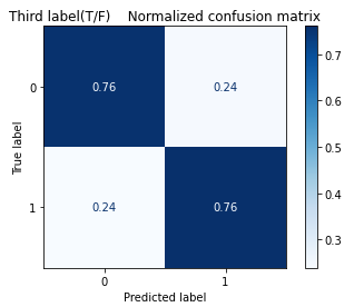
Figure 11. Confusion matrix for the third label (T/F) in linear regression.

As shown in Table 2, the Linear Regression model has an accuracy of ​​0.54. When the dataset is broken into four classifications, the accuracy for the First(I/E), Second(N/S), Third(N/S), and Fourth(J/P) Labels have all gone up to 0.7241, 0.8212, 0.7590, and 0.6542, respectively, as shown in Table 3. The second label shows the most significant improvement among the others.

3.5. Summary tables

Table 2. MBTI types testing set accuracy without separating 4 letters by different methods.

Table 3. Four lettering accuracy compared by six different methods.

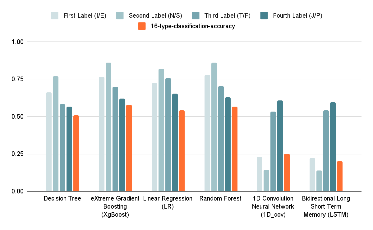
Figure 12. Four lettering accuracy vs. sixteen type classification accuracy in bar chart.

Figure 13. Four lettering accuracy by different methods in bar chart.

3.6. Analysis

In the accuracy result tables and the bar charts in section 3.5, Neural Network type algorithms, such as 1D-CNN and LSTM, perform relatively poorer in the classifications, especially on the First Label and the Second Label classifications.

Such kind of upshot may be due to the following properties of these two neural networks. Both networks are very good at extracting connections between contextual information, but each row of posts in the dataset is made up of a user's 50 most recent posts, and these different posts may not be closely related to each other, or they may not be related at all. In Figure 12, it is clear that decision-tree-related methods outperforms the two neural networks (1D-CNN and LSTM) in any classification. XGBoost and random forest achieved better performance, even better than the basic decision tree. This result may be due to the fact that these methods use strategies such as Bagging and Boosting based on decision trees, which enable the model to perform at a higher level.

In the 4-letter-classification, according to figure 13, one unexpected phenomenon was that the neural network model was more effective in the classification of the latter two letters than the first two, while other methods performed exactly the opposite. This phenomenon is very interesting, and it is probably related to the way features are extracted from different types of models.

4. Conclusion

In this paper, the powerful and effectiveness of the decision tree used for MBTI classification were explored. With the help of the decision tree, this study achieved better performance in terms of classification accuracy compared with that of the traditional CNN and LSTM on the dataset. In the study, decision trees were applied to the classification of four different letters in MBTI. On non-related variance posts, the tree-based method demonstrated excellent performance in feature extraction and MBTI classification when compared with neural networks. The experiment also showed that traditional CNN and LSTM face overfitting problems in the non-related, large number of words, while the tree-based methods can mitigate that phenomenon in the training process.

XGBoost and random forest are integrated decision tree models. They showed an accuracy of more than 75% for the classification of I/E and N/S labels, but this model performs slightly worse for the other two labels. It showed that the decision-tree-related model is efficient in some dimensions of personality measurement, but its accuracy varies in different dimensions. In future research, in order to achieve higher prediction accuracy, this model could be used for predicting the first two labels and another model with a good performance on the last two labels could be combined with it. The new model also achieved an overall accuracy of more than 70 percent on this question, which, while not perfect, showed a general ability to predict personality types. In the follow-up research, more improved decision tree models can be used to achieve higher accuracy.

References

[1]. Gjurković, M., & Šnajder, J. (2018). Reddit: A Gold Mine for Personality Prediction. In Proceedings of the Second Workshop on Computational Modeling of People's Opinions, Personality, and Emotions in Social Media. New Orleans. pp. 87-97. https://aclanthology.org/ W18-1112
[2]. Mylonas, C. (2014). Analysis of networking characteristics of different personality types. Internet Archive. http://arxiv.org/abs/1406.3663
[3]. Xu, X., Zeng, W., Ou, P., & Wang, H. (2018, November). Analysis of medical staff on MBTI personality type test. China Medical Herald, 32:160-163.
[4]. Golbeck, J., Robles, C., Edmondson, M., & Turner, K. (2011). Predicting personality from twitter. 2011 IEEE Third International Conference on Privacy, Security, Risk and Trust and 2011 IEEE Third International Conference on Social Computing. pp. 149-156. https://doi.org/10.1109/PASSAT/ SocialCom.2011.33
[5]. Cui, B.; Qi, C. (2017). Survey Analysis of Machine Learning Methods for Natural Language Processing for MBTI Personality Type Prediction.
[6]. Eng, Zi Jye. (2020). Personality recognition using composite audio-video features on custom CNN architecture. Final Year Project, UTAR.
[7]. Fung, P., Dey, A., Siddique, F. B., Lin, R., Yang, Y., Wan, Y., & Chan, H. Y. R. (2016). Zara the supergirl: An empathetic personality recognition system. Proceedings of the 2016 Conference of the North American Chapter of theAssociation for Computational Linguistics: Demonstrations. pp. 87-91. https://doi.org/10.18653/v1/N16-3018
[8]. Hernandez, R., & Scott, I. K. (2017). Predicting Myers-Briggs Type Indicator with text classification. In Proceedings of the 31st Conference on Neural Information Processing Systems. Long Beach, CA.
[9]. Keh, S. S., & Cheng, I. (2019). Myers-Briggs Personality Classification and Personality-Specific Language Generation Using Pre-trained Language Models. ArXiv, abs/1907.06333.
[10]. Friedman, J. H. (2002). Stochastic gradient boosting. Computational Statistics & Data Analysis, 38: 367-378. https://doi.org/10.1016/S0167-9473(01)00065-2
[11]. Pedregosa, F., Varoquaux, G., Gramfort, A., Michel, V., Thirion, B., Grisel, O., Blondel, M., Prettenhofer, P., Weiss, R., Dubourg, V., Vanderplas, J., Passos, A., Cournapeau, D., Brucher, M., Perrot, M., & Duchesnay, É. (2011). Scikit-learn: Machine Learning in Python. JMLR 12, 12, 2825-2830. https://scikit-learn.org/stable/about.html#citing-scikit-learn
[12]. Sebastian, A. (2020). A Gentle Introduction To Calculating The TF-IDF Values. Towards Data Science. https://towardsdatascience.com/a-gentle-introduction-to-calculating-the-tf-idf-values-9e391f8a13e5
[13]. Chen, T., & Guestrin, C. (2016). XGBoost: A scalable tree boosting system. In Proceedings of the 22nd ACM SIGKDD International Conference on Knowledge Discovery and Data Mining. http://dx.doi.org/10.1145/2939672.2939785
[14]. Lecun, Y., Haffner, P., Bottou, L., & Bengio, Y. (1999). Object Recognition with Gradient-Based Learning. In Shape, Contour and Grouping in Computer Vision. Springer, Berlin, Heidelberg. https://doi.org/10.1007/3-540-46805-6_19
[15]. Hochreiter, S., & Schmidhuber, J. (1997). Long Short-Term Memory. Neural Computation, 9: 1735-1780. https://doi.org/10.1162/neco.1997.9.8.1735
[16]. Brownlee, J. (2016). Linear Regression for Machine Learning. Machine Learning Mastery. https://machinelearningmastery.com/linear-regression-for-machine-learning/
Cite this article
Chen,F.;Shen,X.;Liu,Y.;Wang,Y.;Zhang,Z.;Wang,M. (2023). Myers-Briggs Type Indicator analysis using decision-tree-related methods. Applied and Computational Engineering,2,121-135.
Data availability
The datasets used and/or analyzed during the current study will be available from the authors upon reasonable request.
Disclaimer/Publisher's Note
The statements, opinions and data contained in all publications are solely those of the individual author(s) and contributor(s) and not of EWA Publishing and/or the editor(s). EWA Publishing and/or the editor(s) disclaim responsibility for any injury to people or property resulting from any ideas, methods, instructions or products referred to in the content.
About volume
Volume title: Proceedings of the 4th International Conference on Computing and Data Science (CONF-CDS 2022)
© 2024 by the author(s). Licensee EWA Publishing, Oxford, UK. This article is an open access article distributed under the terms and
conditions of the Creative Commons Attribution (CC BY) license. Authors who
publish this series agree to the following terms:
1. Authors retain copyright and grant the series right of first publication with the work simultaneously licensed under a Creative Commons
Attribution License that allows others to share the work with an acknowledgment of the work's authorship and initial publication in this
series.
2. Authors are able to enter into separate, additional contractual arrangements for the non-exclusive distribution of the series's published
version of the work (e.g., post it to an institutional repository or publish it in a book), with an acknowledgment of its initial
publication in this series.
3. Authors are permitted and encouraged to post their work online (e.g., in institutional repositories or on their website) prior to and
during the submission process, as it can lead to productive exchanges, as well as earlier and greater citation of published work (See
Open access policy for details).