1. Introduction

The connected subgraph of a connected graph with the fewest edges, which must include all of the connected graph's nodes, is called the spanning tree [1]. Additionally, a well-known optimization issue in graph theory is the minimal spanning tree (MST) problem. Given an undirected, weighted graph, the goal of the MST problem is to find a tree that spans all the vertices of the graph with the minimum possible total edge weight. Moreover, it has much realistic meaning. MST is widely used in many fields [2-4]. For instance, in network design, a minimum spanning tree can help to optimize the layout of a network, which is found to be helpful in designing the transportation system in urban and rural areas. Next, this article will cover three algorithms (Kruskal, Prim, and Boruvka) that can solve this problem, showing the very steps of the algorithms in detail [5-7]. Then, by using the method of comparison, the differences and commonalities can be found. Lastly, specific backgrounds for applying these three algorithms will be shown.

2. Kruskal’s algorithm

2.1. Specific steps

Sort all the edges in an ascending order of weight;

Start a loop starting with the edge of the least weight;

For each edge:

If adding it to the current MST won’t create a cycle;

Then add it to the MST;

If n-1 edges have been added, then stop the loop;

(n is the amount of the nodes).

2.2. Applying Kruskal’s algorithm in a specific graph

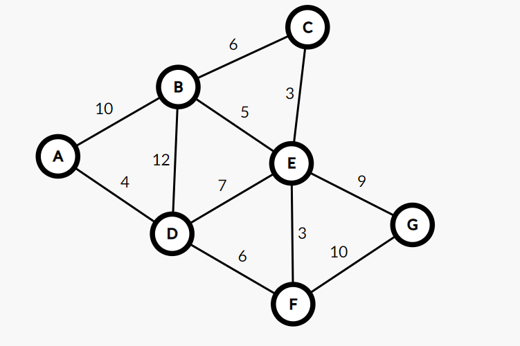
Figure 1. A sample weighted and undirected graph.

Here are the steps of applying Kruskal’s algorithm in the undirected graph above.

The edge with the least weight is CE, and adding it won’t create a cycle. Add CE to the MST.

Next one is EF, and adding it won’t create a cycle. Add EF to the MST.

Next one is AD, and adding it won’t create a cycle. Add AD to the MST.

Next one is BE, and adding it won’t create a cycle. Add BE to the MST.

Next one is DF, and adding it won’t create a cycle. Add DF to the MST.

Next one is BC, and adding it will create a cycle (BC-BE-CE). So, skip BC.

Next one is DE, and adding it will create a cycle (DE-EF-DF). So, skip DE.

Next one is EG, and adding it won’t create a cycle. Add EG to the MST.

Up to now, 6 edges have already been added to the MST. Since there are 7 vertices in the graph, the MST has already been created.

2.3. A universal method to determine whether a cycle will be created

2.3.1. The union-find algorithm. The disjoint-set data structure, sometimes referred to as the union-find algorithm, is a group of techniques that enables us to effectively manage a collection of disjoint sets. Union and find are the union-find algorithm's primary operations.

The find operation takes an element as input and returns the unique identifier of the set that the element belongs to. If two elements have the same unique identifier, then they belong to the same set. Usually, recursion will be applied in this operation.

The union operation takes two sets and merges them into a single set. This operation is accomplished by assigning the identifier of one set to the other merged set.

In terms of a tree, the set is a subtree, and the unique identifier is the root node. The find operation recursively follows the parent node of a node until the root node is found.

2.3.2. The application of the union-find algorithm in this process. For each edge, tell whether its two nodes have the same root node (identifier) with the find operation. If so, it means that the two nodes are already in the same tree. As a result, connecting them with this edge will create a cycle. Consequently, if the two nodes are not in the same tree, then join the edge into the MST and set the one node’s root node to the other node’s root node to join this node to the MST, which is called the union operation.

2.4. Time complexity analysis

The whole algorithm contains two main parts: the sorting and the loop of the edges. Obviously, the time complexity of the latter one is O(n) (n is the number of the nodes) which is absolutely less than the sorting operation. The complexity of the sorting algorithm can reach as low as O (nlogn) by applying quick sort, merge sort, etc. So, the final time complexity is the larger one, O (nlogn).

3. Prim’s algorithm

3.1. Specific steps

Choose a random node as the starting node.

Create a set (named S) of nodes that are not yet in the MST. Initially, this set contains all nodes except the starting node.

For each node in the MST, find the cheapest edge that connects it to a node in S.

Select this node with the cheapest edge and add it to the MST, and remove this node from S.

Repeat steps 3 and 4 until all nodes are in the MST.

3.2. Applying Prim’s algorithm in a specific graph

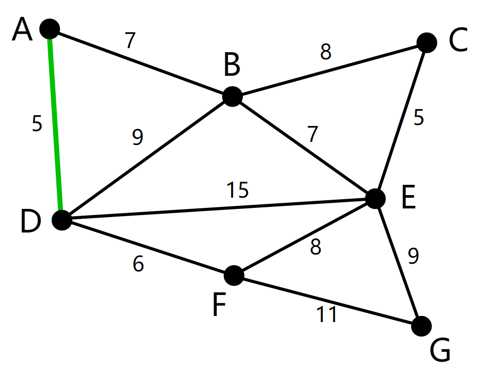
Figure 2. A sample weighted and undirected graph.

Here are the steps of applying Prim’s algorithm in the undirected graph above.

Choose A as the starting node. The set of nodes that are not in the MST yet is S, which contains B, C, D, E, F, and G now.

The cheapest edge connecting MST and S is AD weighted 5, so add AD to MST and remove D from S. The present S is B, C, E, F, and G.

The cheapest edge connecting MST and S is DF weighted 6, so add DF to MST and remove F from S. The present S is B, C, E, and G.

The cheapest edge connecting MST and S is AB weighted 7, so add AB to MST and remove B from S. The present S is C, E, and G.

The cheapest edge connecting MST and S is BC weighted 8, so add BC to MST and remove C from S. The present S is E, and G.

The cheapest edge connecting MST and S is CE weighted 5, so add CE to MST and remove E from S. The present S is G.

The cheapest edge connecting MST and G is EG weighted 9, so add EG to MST and remove G from S. The present S is empty. The algorithm ends.

3.3. Time Complexity analysis

The time complexity of Prim's algorithm is O (n ^ 2), where n is the number of nodes in the graph. However, if a priority queue is used to select the minimum-weight edge at each step, it takes O (log n) time to extract the minimum element. The algorithm repeats this process m-1 times to construct the MST. In conclusion, the total time complexity of the algorithm is O (m log n). (m is the number of edges in the graph.)

4. Boruvka’s algorithm

4.1. Main ideas

Boruvka’s algorithm can be considered as the combination of Prim and Kruskal [8].

For each current connected block, find the shortest edge from this connected block that is not in the minimum spanning tree and reaches other connected blocks.

Add it to the MST.

Repeat this process until the MST is built.

4.2. Specific steps

As we get started, every single node is considered as a connected component itself. We will start the process with them.

Firstly, find the cheapest edge leaving a component by checking all the edges. If one edge meets these restrictions, it has not been used yet, so merging it is not going to create a cycle.

Then find the root node of the tree to which one terminal node belongs, check if the current edge is cheaper than its current cheapest edge. If so, update it. Then do the same thing to the other terminal node of this edge.

After a loop, the cheapest edges of each component can be obtained.

Check all the nodes to merge each cheapest edge if it hasn’t been used before. Once an edge is merged, mark it as used and use the union operation to merge one component with the other.

Repeat the whole process until n-1 edges are merged.

4.3. Applying Boruvka’s algorithm in a specific graph

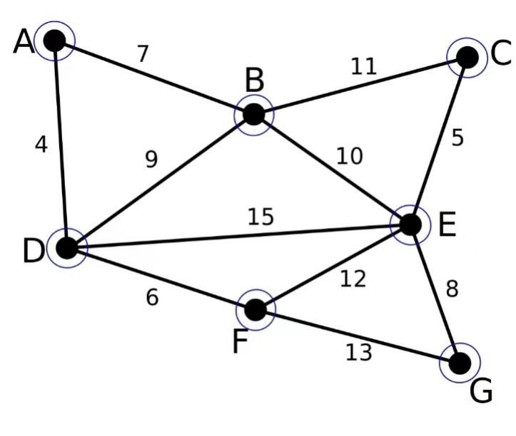
Figure 3. A sample weighted and undirected graph.

Initially, all the nodes are considered as a single component.

Loop all the edges and find the “Best” array.

AB is best for B;

AD is best for A and D;

DF is best for F;

EG is best for G;

CD is best for C and E.

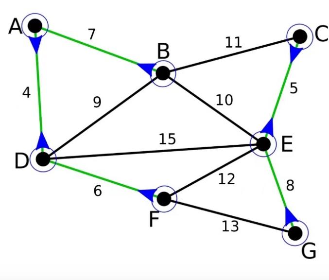
Figure 4. Every “Best” edges are obtained.

Then merge all the connected nodes to a bigger component.

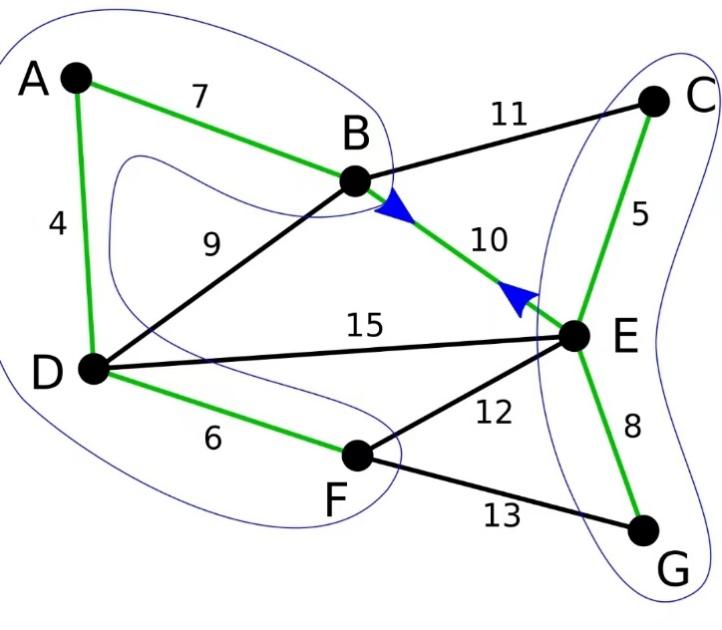
Figure 5. Finding the cheapest edge connecting two blocks.

Loop all the edges and find the “Best” array.

In the all-available edges, BE is the cheapest to connect the two components. Add it to the MST.

Up to now, n-1 edges have been merged, so the MST has been built.

4.4. The application of the union-find algorithm in this process

In Boruvka's algorithm, each node initially belongs to a separate set (tree). During each iteration, the algorithm scans all the edges in the graph and, for each component, finds the cheapest edge that connects it to a node not in the component. To do this efficiently, the algorithm uses the Find operation to determine which component a node belongs to. If two nodes are connected by an edge, the Union operation is used to merge the components containing the two vertices.

The algorithm repeats this process until there is only one component left, which corresponds to the MST. The use of the union-find algorithm allows the algorithm to efficiently determine the components that each node belongs to and to merge components when necessary.

4.5. Time complexity analysis

N nodes need to be merged for log n times; every merging operation is O(m) because every edge needs to be checked to maintain the cheapest edge of each component. So, the total time complexity is O (m log n).

5. The comparison of the three algorithms

Obviously, these three algorithms can reach the same goal with different time complexity. So, it’s necessary to make a judgement about which one should be applied. By observing the formula of each one, the Kruskal's algorithm has a time complexity of O(m log m), where m is the number of edges in the graph, making it appropriate for determining the MST of a sparse graph [9]. Regardless matter how many edges are there in a graph, the Prim method has an O(n^2) computational cost. To determine the MST of a dense graph, the Prim's technique is therefore appropriate [10]. Prim’s algorithm is still outstanding in dense graphs since its time complexity is O (m log n) with the optimizing of priority queue. Boruvka’s algorithm is the same as Prim’s algorithm in terms of time complexity.

Here is the experiment:

Separately generate three sparse graphs randomly, run these three algorithms to find the MST for 1000 times. Then calculate the average runtime.

Table 1. The average runtime of the three algorithms in an example sparse graph.

As the Table 1 shows, Kruskal is much better.

Separately generate three dense graphs randomly, run these three algorithms to find the MST for 1000 times. Then calculate the average runtime.

Table 2. The average runtime of the three algorithms in an example dense graph.

As the Table 2 shows, Prim and Boruvka are better.

6. Conclusion

This paper elaborated the main ideas and implementation steps of three typical MST algorithms and analyzed their time complexity. It also introduced an important algorithm called union-find algorithm and its application in Kruskal’s and Boruvka’s algorithm. In the end, the differences of three algorithms are discussed, indicating their suitable situation. However, it doesn’t talk about the various optimization methods of these algorithms which can result in different time complexity in the end. In the future research, multiple optimization methods of these three algorithms will be taken into consideration and the difference of their efficiency will be also discussed.

References

[1]. R. L. Graham and P. Hell, “On the history of the minimum spanning tree problem,” IEEE Annals of the History of Computing, vol. 7, no. 1, pp. 43–57, 1985.
[2]. T. Mahapatra and M. Pal, “Fuzzy colouring of m-polar fuzzy graph and its application,” Journal of Intelligent and Fuzzy Systems, vol. 35, no. 6, pp. 6379–6391, 2018.
[3]. T. Mahapatra and M. Pal, “An investigation on m-polar fuzzy threshold graph and its application on resource power controlling system,” Journal of Ambient Intelligence and Humanized Computing, vol. 13, no. 1, pp. 501–514, 2022.
[4]. M. Laszlo and S. Mukherjee, “Minimum spanning tree partitioning algorithm for microaggregation,” IEEE Transactions on Knowledge and Data Engineering, vol. 17, no. 7, pp. 902–911, 2005.
[5]. J. B. Kruskal, “On the shortest spanning subtree of a graph and the traveling salesman problem,” Proceedings of the American Mathematical Society, vol. 7, no. 1, pp. 48–50, 1956.
[6]. P. C. Pop, “The generalized minimum spanning tree problem: an overview of formulations, solution procedures and latest advances,” European Journal of Operational Research, vol. 283, pp. 1–15, 2020.
[7]. R. C. Prim, “Shortest connection networks and some generalizations,” Bell System Technical Journal, vol. 36, no. 6, pp. 1389–1401, 1957.
[8]. J. Nesetril, E. Milkova, and H. Nesetrilova, “Otakar Boruvka on minimum spanning tree problem - translation of both the 1926 papers, comments, history,” Discrete Mathematics, vol. 233, no. 1-3, pp. 3–36, 2001.
[9]. H. Li, W. Mao, A. Zhang, and C. Li, “An improved distribution network reconfiguration method based on minimum spanning tree algorithm and heuristic rules,” International Journal of Electrical Power & Energy Systems, vol. 82, pp. 466–473, 2016.
[10]. E. van Dellen, L. Douw, A. Hillebrand et al., “Epilepsy surgery outcome and functional network alterations in longitudinal MEG: a minimum spanning tree analysis,” NeuroImage, vol. 86, no. 1, pp. 354–363, 2014.
Cite this article
Zhang,R. (2023). The comparison of three MST algorithms. Applied and Computational Engineering,17,191-197.
Data availability
The datasets used and/or analyzed during the current study will be available from the authors upon reasonable request.
Disclaimer/Publisher's Note
The statements, opinions and data contained in all publications are solely those of the individual author(s) and contributor(s) and not of EWA Publishing and/or the editor(s). EWA Publishing and/or the editor(s) disclaim responsibility for any injury to people or property resulting from any ideas, methods, instructions or products referred to in the content.
About volume
Volume title: Proceedings of the 5th International Conference on Computing and Data Science
© 2024 by the author(s). Licensee EWA Publishing, Oxford, UK. This article is an open access article distributed under the terms and
conditions of the Creative Commons Attribution (CC BY) license. Authors who
publish this series agree to the following terms:
1. Authors retain copyright and grant the series right of first publication with the work simultaneously licensed under a Creative Commons
Attribution License that allows others to share the work with an acknowledgment of the work's authorship and initial publication in this
series.
2. Authors are able to enter into separate, additional contractual arrangements for the non-exclusive distribution of the series's published
version of the work (e.g., post it to an institutional repository or publish it in a book), with an acknowledgment of its initial
publication in this series.
3. Authors are permitted and encouraged to post their work online (e.g., in institutional repositories or on their website) prior to and
during the submission process, as it can lead to productive exchanges, as well as earlier and greater citation of published work (See
Open access policy for details).