


1. Introduction
Object detection is a fundamental task in the computer field and has a wide range of applications. In self-driving cars, the environment is photographed with a monocular or binocular camera, and object detection technology is used to inspect vehicles and road conditions on the road, deal with complex landforms [1], and identify traffic signals. However, while widely used, object detection technology is also very challenging. The task of object recognition requires not only efficiency but also considerable accuracy. For autonomous vehicles [2], safe driving is a top priority. This is also the bottleneck encountered by the current autonomous driving technology, which has high requirements not only for the accuracy of object recognition but also for the real-time performance of object detection technology. Currently, the vast majority of self-driving cars have difficulty meeting Level 4 autonomous driving requirements [2][3]. The reason is that its safety performance is difficult to guarantee, and the driver must be alert. Every step in the development of object detection technology will promote progress in many fields. Image processing is divided into image preprocessing, feature extraction, feature selection, model establishment, matching, positioning, and other steps.
|
Figure 1. Object detection in autonomous driving. |
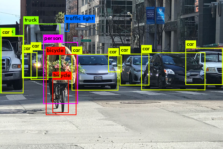
As shown in Figure 1, in autonomous driving, there are three main tasks that require object recognition. Distinguish foreground and background, determine the classification of objects, and determine the location of objects.
As shown in Figure 2, in the decades of development of obstacle detection, there have been many important milestones, among which, in 2012, deep learning technology began to be widely used in object detection [4]. Especially with the rapid development of hardware equipment in recent years. Especially with the development of the Graphics Processing Unit (GPU), deep learning networks are developing more vigorously. Taking 2012 as the boundary, object recognition technology can be divided into traditional detection methods and deep-learning-based detection methods. Among them, the traditional detection algorithms are represented by HOG Detector and Deformable Part-Based Model (DPM) [5] [6]. However, due to their processing speed and accuracy, they are not as good as the detection method based on deep learning. The current mainstream algorithms are divided into one-stage detectors and two-stage detectors. The representative of one-stage detectors is the You Only Look Once (YOLO) algorithm proposed by Joseph Redmon and others, and the representative of two-stage detectors is the Region-Based Convolutional Neural Network (R-CNN) series proposed by Ross Girshick [7][8]. This article will focus on the comparison and analysis of these algorithms.
This paper will briefly introduce some important traditional methods of object detection in the second part. It will focus on three important methods before deep learning: SIFT, stereo with graph cuts, and the HOG detector. In the third part, the idea of the YOLO algorithm will be introduced, and several algorithms from the YOLO series will be analyzed. In the fourth part of the paper, the algorithms of the R-CNN series are introduced, including Fast R-CNN and Faster R-CNN. Part 4 introduces the SSD method. Then, the above algorithms will be analyzed and compared, and a summary will be made.
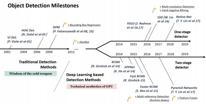 Figure 2. Milestones of object detection.
2. Traditional detection methods
Before the deep-learning era, there were many important methods, which are important milestones in the development of object recognition technology so far. SIFT, stereo with graph cuts, and the HOG detector are three representative traditional object recognition methods. These three approaches have a place even now in deep learning, even though deep learning techniques have profoundly changed object recognition.
2.1. SIFT
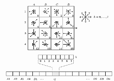
Scale-invariant feature conversion (SIFT) is a computer vision algorithm that is used to detect and explain local features in an image. It detects the extrema of the spatial scale and extracts its position, scale, and rotation invariants. This algorithm was published by David Lowe in 1999 and completed in 2004 [9][10]. The detection rate of partial object occlusion using SIFT feature descriptions is also very high, and more than three SIFT object features are sufficient to calculate position and orientation. Under current computer hardware speeds and small feature database conditions, recognition speeds can be close to real-time computation. The SIFT feature has a large amount of information and is suitable for fast and accurate matching in large databases. As shown in Figure 3, the core of this algorithm is to calculate the descriptor of local images. For example, a 16*16 window is set to a keypoint, and then it is divided into 16 4*4 blocks. For these blocks, an 8-bin orientation histogram is created.
|
Figure 3. SIFT structure. |
The essence of the SIFT algorithm is to find keypoints (feature points) in various scale spaces and calculate the direction of the keypoints. The important points detected by SIFT are very prominent points that do not change due to factors such as lighting, affine transformations, and noise, for example, corner points, edge points, bright spots in dark areas, dark spots in bright areas, and so on.
2.2. Stereo with graph cuts
Stereo with graph cuts was proposed in 1998 [11]. Graph cutting techniques have been used to solve the stereo matching problem involving global constraints. These methods transform the matching problem into the minimization of a global energy function. The minimization is achieved by finding the optimal cut (of minimum cost) in a special graph. Due to the max-flow min-cut theorem, determining a min-cut on a graph representing a flow network is equivalent to computing a max-flow on the network. In order to construct a flow network with positive weights such that the cost C of each cut C of the network is equal to an additional constant, we give a Boolean value.
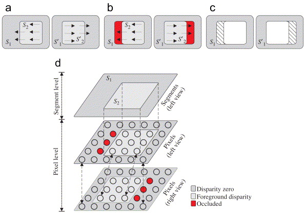
Then the minimum cut of the global optimal through the computational graph can be obtained in polynomial time. The mapping between cuts and variable assignments is done by representing each variable in the graph with a node. Given a cut, each variable has a value of 0 if the corresponding node belongs to a component connected to the source. If it belongs to the component connected to the source, and 1 belongs to the component connected to the sink. Figure 4 shows the basic method of stereographic cutting [12]. Two stereo pair images are obtained in Fig. 4a. The image on the left shows two clips, and the view on the right shows the corresponding clips. The segment is slightly biased in the right view, while the segment has zero disparity (the red part in Figure 4 (b)). If using the correct disparity to match the full segment of the left image in the right view, this will result in expensive matching of these occluded regions. These regions are marked with shading in the left view of Figure 4 (c). Due to occlusion issues, it is possible to be assigned to the wrong disparity model, showing lower matching costs. When modeling the problem only at the segment level, it can be easily identified that the segment has zero variance. However, in addition to this, the occluded part should be considered to correctly match the second view with zero disparity. So the correct statement must be: have zero parallax but contain a set of occluded pixels. Therefore, occlusion detection requires the participation of the pixel domain.
|
Figure 4. Graph-cut-based stereo. |
2.3. HOG detector
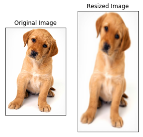
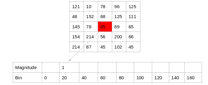
HOG is the abbreviation of the Histogram of Oriented Gradients algorithm, proposed by Navneet Dalal and Bill Trigg in 2005 [13]. HOG is good at manipulating the shape of objects. The core idea of HOG is that the detected local object shape can be described by the distribution of the light intensity gradient or edge direction. In this case, its algorithm was superior to all edge detection algorithms at the time. It is characterized by focusing on the gradient of image regions and the size of different regions in the image. The method of implementation is to first adjust the image to a fixed size. Navneet Dalal and Bill Trigg chose to adjust it to 128*64 pixels in the paper, as shown in Figure 5. Then, the gradient parameters are calculated according to the angle of the image. After getting the gradient of the image, divide it into 8*8 grid cells. For each block cell, nine histograms are generated, and bin values are generated among them. The bin size shown in Figure 6 is 20. By doing this, nine matrixes for each grid cell can be obtained. Then the frequency of orientation is put into the matrix. Take the array as a bin for the block and append the values of Vj and Vj+1 to the indices of the jth and (j+1)th bins calculated for each pixel in the array. Normalization is performed to reduce the effect of contrast changes between images. The final result is 7*15*36 HOG features.
|
Figure 5. Preprocess of the image. |
|
Figure 6. Create histograms using gradients and orientation. |
3. YOLO series
3.1. Methodology of YOLO
YOLO (You Only Look Once) is a one-stage detection algorithm that solves object detection as a regression problem, that is, finding eigenvalues and frames in a network. YOLO is based on a single end-to-end network that completes the input from the original image to the output of object location and category.
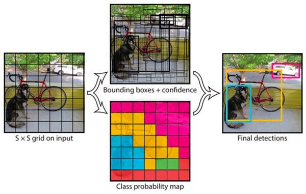
In the process of image information processing, Joseph Redmon and his team first divide the image into 19*19 grid cells. Apply an image classification algorithm to each grid cell [7]. Among them, for each grid cell, the training label is defined as 8 parameters: y = {p_c, b_x, b_y, b_h, b_w, c_1, c_2 , c_3}, where p_c indicates whether there is a target detection object in this grid cell. 0 means no, 1 means yes. b_x and b_y represent the horizontal and vertical coordinates of the target object in the grid cells where it is located; b_h and b_w represent the length and width of the detected object, respectively; and c_1, c_2, and c_3 represent what the detected object is. Then assign this object to the grid cells where it is located.
|
Figure 7. Simple illustration of YOLO. |
The input image goes through a convolutional neural network to achieve the task of feature extraction. Then, the feature maps are output; in the program I reference, it is a 7*7*1024 feature map [7]. The fully connected layer is used to process the feature map so as to obtain the parameters of the type and position of the object in each grid cell. The network structure characteristics of YOLOv1 draw on GoogLeNet. In YOLOv1, there are 24 convolutional layers and two fully connected layers. At that time, it was a very popular method for video detection. At the time of testing, the class information and bounding box predicted by each grid are multiplied by the predicted confidence information to get the class-specific confidence score of each bounding box. After getting the prediction box of each bounding box, set a threshold to filter the low-scoring options. Then normalize the remaining bounding boxes to get the final result.
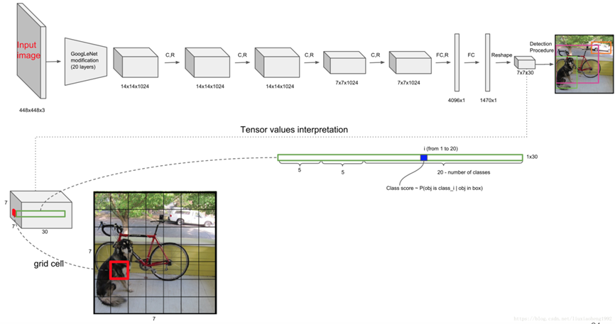
Figure 8. YOLO network structure.
In terms of the design of the loss function, the overall idea of Joseph Redmon and his team is to use squared error loss for architecture. YOLOv1 gives greater weight to 8-dimensional coordinates, which means that prediction errors in small bounding boxes are more intolerable in comparison. Larger bounding boxes are given smaller weights. In addition, the division of labor is also carried out for multiple bounding boxes. For the bounding box with a larger predicted IoU value, it is responsible for detecting the value in the grounding truth. Also known as the specialization of bounding box predictors in the text.
YOLO completes the prediction of bounding boxes and categories for all objects in the image in one network model, avoiding spending a lot of time generating candidate regions. Its strengths are detection speed and recognition capabilities, rather than perfectly locating objects.
3.2. The network improvement of the next versions
|
Figure 9. Network structure of YOLOv2. |
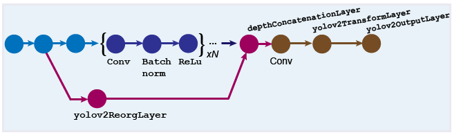
The core network structure of YOLOv2 is called Darknet-19, a network named by Joseph Redmon and his team [14]. An important improvement in v2 is the addition of a BN layer (batch normalization). The advantage of this is that a batch normalization layer is added to each layer of the network, which normalizes the input of each layer, making convergence easier. The fully connected layer is also removed in v2, and the anchor box is used to perform this function. Different from the two prior boxes in each grid cell in YOLOv1. The YOLOv2 version uses clustering to extract prior boxes. Clusters the boxes in the true figure coordinates of all the labeled data. The method of classification refers to K-means clustering.
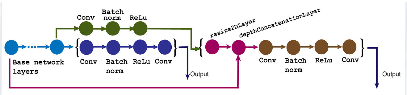
The biggest improvement in YOLO v3 is the network architecture [15]. YOLOv3 uses Darknet-53, named by Joseph Redmon and his team. Compared with v2, the number of network layers has increased. Multiscale is also the most important improvement in the YOLOv3 version. The three corresponding candidate boxes also correspond to small, medium, and large, respectively. Each feature map corresponds to three sizes of candidate boxes. YOLOv3 is different from the traditional image pyramid. Traditional image pyramids resize the image to get a controllable feature map size. But YOLO has made improvements in the pursuit of speed. Then upsample the 13*13 feature map to a 26*26 feature map, which is then added to the 26*26 feature map output by the previous layer to complete the fusion. 52*52 feature map fusion is the same. YOLOv3 borrows the idea of ResNet so that accuracy can be improved by stacking more layers. More useful for feature extraction. Residual links are used in most networks today. Through residual linking, better features can be obtained.
The advantage of YOLOv4 is that it can train on a GPU with better training results without necessarily requiring expensive TPUs and other equipment [16]. The main improvement is reflected in the data level and network structure. YOLOv4 proposes a bag of freebies (BOF). This approach implements data augmentation functions at the data level. This process can improve the training effect but does not affect the test speed. The traditional basic methods of data augmentation include adjusting brightness, contrast, hue, flip scaling, etc. But one method explained in this article is mosaic data augmentation. Stitch the four images into one whole image for training. The four images are each enhanced according to the original method and then stitched together. In addition, there is random erase, which refers to replacing parts of the graph with random values. And hide and seek, which randomly obscures local images. YOLOv4 also uses self-adversarial training (SAT) to improve the training effect by adding noise points. The label smoothing method was proposed in YOLOv4. Adjust the label's data to make it smoother. Replace 0 and 1 with 0.05 and 0.95. It makes the network have a better anti-overfitting process. Use to make the clustering tighter. But the fault tolerance will also improve, and the clusters will be more separated.
|
Figure 10. Network structure of YOLOv3. |
|
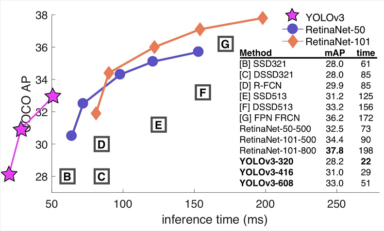
Figure 11. Comparison among YOLOv3 and other methods. |
3.3. 3YOLOv5: the state-of-the-art method
YOLOv5 is more focused on engineering-level applications. In terms of network structure and algorithm, it is not much different from V4, but it has a better effect in practical application.
YOLOv5 uses the same mosaic data augmentation method as YOLOv4 in the input. In the COCO dataset trained by YOLOv5, the proportion of small images is higher. Therefore, using the mosaic enhancement method has a better detection effect. There is also an adaptive scaling of the image size, which makes processing faster.
In the backbone part, YOLOv5 has an important improvement, which is the introduction of the Focus structure, which enables the network to perform slicing operations.
The CSP net structure is introduced in both the neck and backbone of YOLOv5. And YOLOv4 only uses the CSP structure in the backbone network. This can reduce the memory cost, make the CNN network more fault-tolerant, and improve the network’s learning ability.
In Yolov5, CIOU_Loss is used as the loss function of the bounding box. This is the same as its previous version.
4. Region based convolutional neural networks(R-CNN)
|
Figure 12. Simple illustration of R-CNN. |
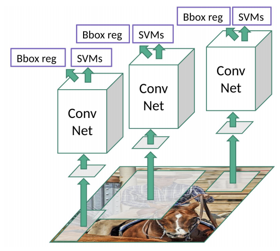
The representatives of two-stage detection are the RCNN series. It differs from one-stage detection in that it generates some region proposals in the first stage of detection [17]. Then the second stage is detecting each region’s proposal, whether it is a cat, a car, etc. There are two main problems that need to be solved: classification and regression. The process of object detection is a regression process. It is trained on the basis of comparing the values of the bounding box and ground truth to realize the regression problem, that is, solving for the coordinate values of a bounding box containing an object. The classification of objects belongs to logistic regression. Before that, its challenge was the effect of multi-object detection. The first step is to select RoI (region of interest), which is almost the same as the anchor box I mentioned in the YOLO series. In the RCNN method, the way to select the candidate bounding box is through the method of selected search. This is a classic method for selecting IoU. Through the selected search method, about 2000 RoIs can be obtained. But the 2000 RoIs obtained at this time are different in shape and size, and the CNN network has a limit on the image size. Therefore, a process is required to make the input RoIs of the same size. Two different methods are mentioned in the paper: anisotropic scaling and isotropic scaling. In order to overcome the problem of too little labeled training data, supervised pre-training is used in the paper. Compared with the VGG network, although the accuracy of Alexnet is not as good as that of the VGG network, it saves about 2/3 of the calculation amount. The feature extraction part of Alexnet includes five convolutional layers and two fully connected layers. In Alexnet, the number of neurons in the p5 layer is 9216, and the number of neurons in f6 and f7 is 4096. After training through this network, each input candidate frame picture can get a 4096-dimensional feature vector. Perform fine-tuning training on the RoI selected by the selected search. If there are N types of objects to be detected, the last layer of pre-training is replaced by one more output neuron. Then there is the problem of binary classification. Ross Girshick and his team set the threshold of IoU at 0.3, and when the IoU is less than 0.3, it will be set as a negative sample [17]. Otherwise, it was set as a positive sample. Once the CNN f7 layer features are extracted, the model will train an SVM classifier for each object. When using CNN to extract 2000 candidate boxes, a feature vector matrix such as 2000*4096 can be obtained, and then multiply such a matrix with the SVM weight matrix 4096*N (N is the number of classification categories; because N SVMs were trained, each SVM packs 4096 W).
4.1. Fast R-CNN
|
Figure 13. Simple illustration of fast R-CNN. |
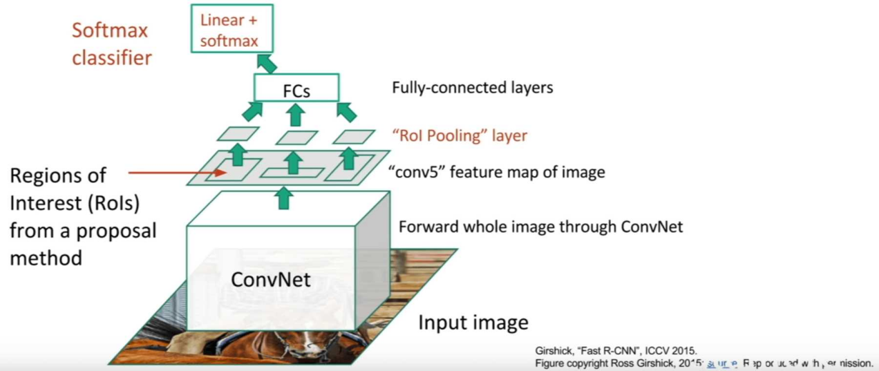
Through the interpretation of RCNN above, it is easy to see that there are many problems. The first problem is that the whole process is implemented in three steps. First, it requires generating 2000 RoIs and then using BBox regression to locate the coordinates of the object. Then, the classification of objects is achieved through SVMs. In other words, RCNN needs to go through the candidate box search stage, the CNN feature extraction stage, and the SVM training stage. The second problem is that it consumes a lot of time and memory. For the training of SVM and bound-box regressors, each proposed feature is proposed and stored on the disk. The storage of these features often requires hundreds of gigabytes of storage space and takes a long time. In the test phase, since the 2000 RoIs generated by the selected search have to be convolved, the repeated operation is very cumbersome. According to the data in the paper, it takes 47 seconds to detect a whole picture with VGG16, which obviously cannot meet the needs of real-time detection [8]. Since all 2000 region proposals need to be convolutional, this process cannot share computation, resulting in a lot of repeated computations. Fast R-CNN was proposed by Ross Girshick and his team. Unlike several convolutions in RCNN, fast R-CNN has only one overall convolution. The RoI max pooling layer is to divide the RoI window with the original size of h*w into the grid size of H*W. And then in each channel-independent max-pooling is performed in the small grid range to obtain features of dimension H * W number of channels. After passing through the ROI pooling layer, the feature map sizes are equal, and then the FC layer can be connected. This greatly improves efficiency. The overall input of Fast R-CNN is the RoI information selected using the selected search algorithm. After multiple pooling and convolution, the RoI is on the feature map, and then it is sent to the single-layer pyramid pooling layer to get a feature map of uniform size. After two FC layers, do regression. Although accuracy and efficiency have been greatly improved, there is still a big deficiency. Especially when it comes to training.
4.2. Faster R-CNN
|
Figure 14. Simple illustration of faster R-CNN. |
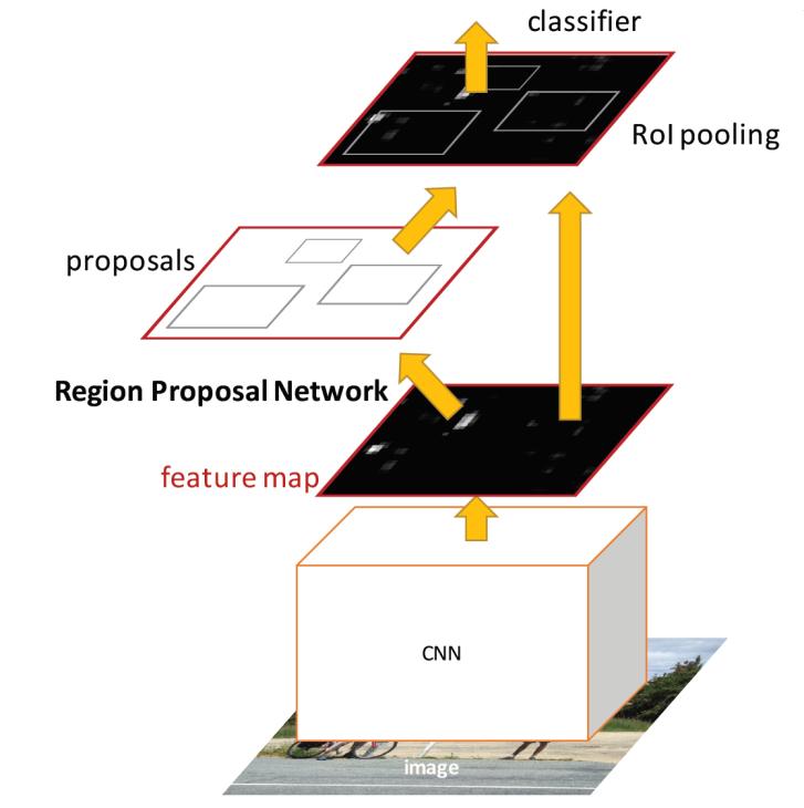
Faster RCNN was proposed in 2017 in order to solve the problem that the processing speed of RCNN is too slow to realize real-time detection. Faster RCNN is currently the best method in this series [18]. The first part obtains the RoI of the detected object, followed by a binary classification of foreground and background. Objects in the RoI are then classified. The core improvement of Faster RCNN is the Region Proposal Network (RPN). The first thing that RPN has to do is obtain the interval area, and the sliding window method is used here. If the input feature is regarded as an image, then for each position of the image, nine anchor boxes are considered: three kinds of areas and three kinds of scales. After that, two full-connection operations are performed, respectively, to obtain 2k classification results and 4k prediction results. Here, k refers to the number of anchors, but it is specified as 9 in Faster R-CNN. Therefore, in the Faster R-CNN, it requires returning 18 classification scores and 36 prediction results. It is noteworthy that the 18 classification score values returned by the RPN network refer to the probability of foreground (object) and the probability of background. The 36 prediction results pertain to 9 sets of deviations from the primary image, with 4 in each set. Sampling is executed after the RPN's loss function. All contenders having IoU greater than 0.7. First, the region proposals are generated in the feature map, and then the region proposals are classified into two categories. Determine whether it is an object or a background, and then perform the regression of the region proposal to ground truth. Classify again to determine what the specific object is.
Same as fast R-CNN, faster RCNN also uses VGG16 or ResNet101 as the class to extract the whole image. Then through the RPN network, the RPN network is the abbreviation of Region Proposal Networks. Finally, RoI pooling and classification network: classify the candidate boxes and fine-tune the anchor box coordinates again (in RPN, the network will adjust the coordinates according to the previously artificially set anchor frame, so here is the second adjustment). Output the detection result. The input to the RPN network is the feature map extracted from the original image by the feature extraction network (VGG or ZF) in Fast R-CNN.
The result is much faster than the fast R-CNN algorithm. However, most faster R-CNN algorithm implementations are still much slower than the YOLO algorithm.
5. Comparison
For YOLO and RCNN in the car type recognition comparison. According to the experiment conducted by Jeong-ah Kim et al., in this experiment, YOLO V4 and Inception V2 models were selected for Faster-RCNN [19]. The dataset for this experiment is divided into vehicles such as light vehicles, sedans, compacts, and large sedans. Most of the experimental data is for cars and small trucks. In this process. According to the experimental results, it shows that R-CNN is better than YOLO in overall accuracy due to its two-stage detection. But in mini-van, sedan, and compact models, YOLO outperforms Faster RCNN in accuracy. Especially for compact cars, YOLO's accuracy is much higher than that of Faster RCNN. But YOLO's FPS is much higher than Faster RCNN. Among them, the FPS of YOLO V4 is 82.1, and the FPS of Faster R-CNN is 36.32. More than doubled.
Table 1. The performance based on YOLO V4.
Label | Average Precision | True Positive | False Positive |
car | 98.08% | 273 | 25 |
mini_van | 94.93% | 52 | 5 |
big_van | 100.0% | 8 | 0 |
mini_truck | 99.04% | 162 | 4 |
truck | 98.52% | 27 | 5 |
compact | 98.59% | 36 | 1 |
Table 2. The performance based on Faster R-CNN.
Label | Average Precision | True Positive | False Positive |
car | 93.2% | 262 | 17 |
mini_van | 87.2% | 52 | 41 |
big_van | 100.0% | 8 | 1 |
mini_truck | 99.7% | 164 | 16 |
truck | 100.0% | 27 | 2 |
compact | 80.3% | 25 | 10 |
Therefore, in this experiment of vehicle detection on the road, we can see that the YOLO algorithm outperforms Faster R-CNN in terms of real-time performance in the experimental results. But the accuracy of Faster RCNN is slightly higher, but the FPS value of YOLO V4 is far better than that of Faster RCNN. Therefore, in autonomous driving, the YOLO algorithm can better complete real-time detection tasks.
|
Figure 15. A comparison of the detection effect. |
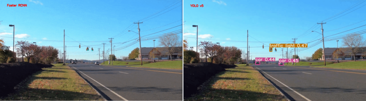
In the experiment conducted by Priya Dwivedi, the video information of the autonomous driving environment was tested on the NVIDIA 1080 Ti, where Faster R-CNN ran nearly twice as fast as YOLO v5 [20]. But for the detection of small objects like traffic lights, YOLO's detection effect is better than Faster R-CNN. This is also reflected in the fact that YOLO's recognition effect is better in the case of people with small car targets when the car is coming from a distance or from a close distance.
6. Conclusion
As shown, YOLO still outperforms FASTER RCNN in many ways. Faster R-CNN has higher accuracy mAP, a lower missed detection rate recall, but slower speed. On the contrary, YOLO is fast, but the accuracy and missed detection rate are low. In practice, most faster R-CNN algorithm implementations are still much slower than the YOLO algorithm.
Still, there is room for improvement in accuracy and efficiency. There are also many popular ways to improve accuracy now, for example, image pyrid, network architecture, feature mix-up, lightweight network design, model compression and quantization, and numerical acceleration technology.
References
[1]. A.de la Escalera et.al.,”Traffic sign recognition and analysis for intelligent vehicles”Volume 21, Issue 3,Volume 21, Issue 3,2003
[2]. I Barabás et al.,”Current challenges in autonomous driving”,IOP Publishing Ltd,2017
[3]. Xiaozhi Chen et al. ,”Monocular 3D Object Detection for Autonomous Driving”,Proceedings of the IEEE Conference on Computer Vision and Pattern Recognition (CVPR), 2016, pp. 2147-2156,2016
[4]. Zhong-Qiu Zhao et al.,”Object Detection With Deep Learning: A Review”, IEEE Transactions on Neural Networks and Learning Systems (Volume: 30, Issue: 11, 2019
[5]. Navneet Dalal et al. “Histograms of oriented gradients for human detection”
[6]. P Felzenszwalb et al.” A discriminatively trained, multiscale, deformable part model”
[7]. Joseph Redmon et al.” You Only Look Once:Unified, Real-Time Object Detection”
[8]. Ross Girshick et al. “Fast R-CNN”
[9]. David G. Lowe ”Object Recognition from Local Scale-Invariant Features”
[10]. Lowe, David G. “Distinctive image features from scale-invariant key points. ”
[11]. Sébastien Roy , Ingemar J. Cox “A Maximum-Flow Formulation of the N-camera Stereo Correspondence Problem”
[12]. MichaelBleyer , Margrit Gelautz “Graph-cut-based stereo matching using image segmentation with symmetrical treatment of occlusions”
[13]. Navneet Dalal , Bill Triggs “Histograms of Oriented Gradients for Human Detection”
[14]. Joseph Redmon et al.” YOLO9000: Better, Faster, Stronger”
[15]. Joseph Redmon et al.” YOLOv3: An Incremental Improvement”
[16]. Alexey Bochkovskiy et al.” YOLOv4: Optimal Speed and Accuracy of Object Detection”
[17]. Ross Girshick et al. “Rich feature hierarchies for accurate object detection and semantic segmentation Tech report (v5)”
[18]. Shaoqing Ren et al. Faster R-CNN: Towards Real-Time Object Detection with Region Proposal Networks”
[19]. Jeong-ah Kim et al. “Comparison of Faster-RCNN, YOLO, and SSD for Real-Time Vehicle Type Recognition”
[20]. Priya Dwivedi. “YOLOv5 compared to Faster RCNN. Who wins?”
Cite this article
Hou,B. (2023). Theoretical analysis of the network structure of two mainstream object detection methods: YOLO and Fast RCNN. Applied and Computational Engineering,17,213-225.
Data availability
The datasets used and/or analyzed during the current study will be available from the authors upon reasonable request.
Disclaimer/Publisher's Note
The statements, opinions and data contained in all publications are solely those of the individual author(s) and contributor(s) and not of EWA Publishing and/or the editor(s). EWA Publishing and/or the editor(s) disclaim responsibility for any injury to people or property resulting from any ideas, methods, instructions or products referred to in the content.
About volume
Volume title: Proceedings of the 5th International Conference on Computing and Data Science
© 2024 by the author(s). Licensee EWA Publishing, Oxford, UK. This article is an open access article distributed under the terms and
conditions of the Creative Commons Attribution (CC BY) license. Authors who
publish this series agree to the following terms:
1. Authors retain copyright and grant the series right of first publication with the work simultaneously licensed under a Creative Commons
Attribution License that allows others to share the work with an acknowledgment of the work's authorship and initial publication in this
series.
2. Authors are able to enter into separate, additional contractual arrangements for the non-exclusive distribution of the series's published
version of the work (e.g., post it to an institutional repository or publish it in a book), with an acknowledgment of its initial
publication in this series.
3. Authors are permitted and encouraged to post their work online (e.g., in institutional repositories or on their website) prior to and
during the submission process, as it can lead to productive exchanges, as well as earlier and greater citation of published work (See
Open access policy for details).
References
[1]. A.de la Escalera et.al.,”Traffic sign recognition and analysis for intelligent vehicles”Volume 21, Issue 3,Volume 21, Issue 3,2003
[2]. I Barabás et al.,”Current challenges in autonomous driving”,IOP Publishing Ltd,2017
[3]. Xiaozhi Chen et al. ,”Monocular 3D Object Detection for Autonomous Driving”,Proceedings of the IEEE Conference on Computer Vision and Pattern Recognition (CVPR), 2016, pp. 2147-2156,2016
[4]. Zhong-Qiu Zhao et al.,”Object Detection With Deep Learning: A Review”, IEEE Transactions on Neural Networks and Learning Systems (Volume: 30, Issue: 11, 2019
[5]. Navneet Dalal et al. “Histograms of oriented gradients for human detection”
[6]. P Felzenszwalb et al.” A discriminatively trained, multiscale, deformable part model”
[7]. Joseph Redmon et al.” You Only Look Once:Unified, Real-Time Object Detection”
[8]. Ross Girshick et al. “Fast R-CNN”
[9]. David G. Lowe ”Object Recognition from Local Scale-Invariant Features”
[10]. Lowe, David G. “Distinctive image features from scale-invariant key points. ”
[11]. Sébastien Roy , Ingemar J. Cox “A Maximum-Flow Formulation of the N-camera Stereo Correspondence Problem”
[12]. MichaelBleyer , Margrit Gelautz “Graph-cut-based stereo matching using image segmentation with symmetrical treatment of occlusions”
[13]. Navneet Dalal , Bill Triggs “Histograms of Oriented Gradients for Human Detection”
[14]. Joseph Redmon et al.” YOLO9000: Better, Faster, Stronger”
[15]. Joseph Redmon et al.” YOLOv3: An Incremental Improvement”
[16]. Alexey Bochkovskiy et al.” YOLOv4: Optimal Speed and Accuracy of Object Detection”
[17]. Ross Girshick et al. “Rich feature hierarchies for accurate object detection and semantic segmentation Tech report (v5)”
[18]. Shaoqing Ren et al. Faster R-CNN: Towards Real-Time Object Detection with Region Proposal Networks”
[19]. Jeong-ah Kim et al. “Comparison of Faster-RCNN, YOLO, and SSD for Real-Time Vehicle Type Recognition”
[20]. Priya Dwivedi. “YOLOv5 compared to Faster RCNN. Who wins?”