1. Introduction

According to people's experience of buying air tickets, it can be found that the price of flights has always been changing, and airlines are also constantly improving the complexity of technology to determine flight pricing based on various factors [1, 2]. Generally speaking, the price of an air ticket depends on departure and arrival time, season, airline, aircraft seat selection and whether there is a transit station. In order to achieve higher profitability, airlines usually use complex pricing models to determine prices and change ticket prices in real time according to actual conditions. Therefore, it is difficult for passengers to buy low-priced air tickets. In order to solve this problem, machine learning-based models are widely used to predict air ticket prices.

Janssen, Dijkstra and Abbas compared four linear regression models and selected the best linear quantile mixed model regression, which predicts air ticket prices according to the remaining days before departure and obtains better fitting curve [3]. Papadakis achieved accuracy rates of 74.5%, 69.9%, and 69.4% respectively through Ripple Down Rule Learner, Logistic Regression, and Linear SVM model predictions [4]. Ren, Yang and Yuan studied Linear regression, Naive Bayesian, SoftMax and SVM models, and found that the correct rate of prediction was between 70% and 80%. Among them, the correct rate of the SVM model using two bins increased to 80.61%. And it is proposed that if more variables are used to train the model, the prediction result with higher accuracy may be obtained [5]. Groves and Gini built an algorithm based on partial least squares regression to predict the best time to buy air tickets [6].

While predicting air tickets, think can be also reversed. Considering how to complete a ticket pricing model and predict ticket prices more accurately based on the features used in the pricing model is also a method to improve the ticket prediction model. For example, Chen and Farias used the incremental learning method to construct a pricing mechanism called robust pricing according to the specified flight route, date, and flight information [7], which controlled the price fluctuation range and ensured that the airline's profits would not suffer significant loss.

The focus of these flight price predictions above is that the model used is a typical machine learning model, and the use of advanced technology on air ticket price prediction issues still needs to be continuously explored. The paper’s key contribution is to use a supervised learning model, and use ensemble learning on the basis of a typical single machine learning model for factors that are generally not strongly correlated, combine multiple models for prediction, and improve the generalization ability of the model.

2. Method

2.1. Dataset

The dataset called “Flight Price Prediction” comes from Kaggle, which includes training file and test file. In order to increase the diversity of the data set segmentation, this experiment merges the two files and re-segments them in subsequent operations. The combined dataset has a total of 13354 data and contains 11 variables which are airline, date of journey, source, destination, route, departure time and arrival time, supplementary information, and price.

The first ten variables both relate to price forecasting. Therefore, this step is to preprocess them. To ensure the accuracy of prediction, the data containing null values should be removed by the entire row. The rest of data can be found that most of variables are composed of strings, so the next step needs to convert them into integer types according to content of the strings. The following are processes of extracting and transforming data features. 1) Remove the date information in “Arrival Time”. 2) Split the attribute “Date of Journey” into “day”, “month”, “year”, and the do same operation on “Arrival Time”, “Dep Time”, split them into “hour”, “minute”. 3) Remove null values and error values from “Duration”, extract “hour” and “minute” from “Duration” and transform them from strings into integer, the resulting “hour” and “minute” data are finally calculated and stored as “Duration” in minutes. 4) Replace the content in “Total Stops” with number, where the number indicates the number of stops on the schedule of flight. 5) Assigns each category in the rest attributes which composed by strings and establishes a one-to-one mapping relationship between numbers and feature attributes.

2.2. Models

2.2.1. Ridge regression. Ridge regression is a regularized use of linear regression and prolongation of linear regression. When ordinary linear Regression models deal with multiple linear regression problems, the least squares method is usually used. The approximate solution is:

\( \hat{β}(λ)={({X^{T}}X)^{-1}}{X^{T}}y) \) (1)

However, when the data has multiple variable collinearities and the matrix is not a full-rank matrix which also means X^TX is irreversible, there will be multiple least square solutions. In order to solve this problem, Hoerl and Kennard introduces a regularization term to make β have a solution [7]. To solve the multicollinearity problem of data attributes, the specific method is as follows: increase the penalty for the coefficient value on the basis of the sum of squared residuals calculated by the standard linear regression model:

\( \hat{β}(λ)={({X^{T}}X+λI)^{-1}}{X^{T}}y) \) (2)

\( λ \) in the formula is the ridge coefficient, and \( I \) is the identity matrix. The introduction of \( λI \) can be used to limit the size of the regression coefficient, thereby effectively controlling the fitting degree of the model. Therefore, the ridge regression model was chosen as the experimental model. In this paper, the selection of model parameters for ridge regression is based on the combination of the best parameters obtained by grid search. The regularization parameter alpha=2.0 is used to control the weight of the regularization term in the objective function. Using the singular value decomposition method as the solution method solver=’svd’. The model scored 0.42767 on the training data and 0.45180 on the test set. Although the test set scores better than the training set, neither shows good predictive result.

2.2.2. Random forest regressor. The random forest regression model composed of multiple unrelated regression trees is a typical ensemble learning. All the trees in the forest form a set of metrics, which are filtered and applied layer by layer from root to leaf, and finally predict the input [8]. The stages for the random forest regression algorithm are approximately as follows. 1) Randomly select m sample points in the training set S for sampling with replacement. 2) Randomly select k features in the original training set, and this k is used for feature division of decision tree nodes. Usually k=sqrt(p), where p is the number of original features. 3) Build a decision tree using (1) selected samples and (2) selected features. The decision rules are established by dividing the sample characteristics, and the Gini impurity or entropy is used as the division standard in each stage, and the best division features and division points are selected. 4) Repeat the first three steps to build multiple decision trees. For each decision tree, sample selection and feature selection are repeated, so each tree is independent. 5) The ultimate result of the prediction is obtained by averaging the predictive results for each tree in the random forest.

When using this function in this article, a grid search is used for parameter selection. The number of decision trees is 200. The maximum depth of the tree is 20. For node division, 2 samples are the bare minimum needed, when the number of samples of a node is less than this value, the node becomes a leaf node and will not be split. The larger the value, the smaller the subtree, which may lead to overfitting of the model.

one sample is the very minimum needed for a leaf node, when the number of samples of any child node after the node is split is less than this value, the split operation will not be performed, and the node becomes a leaf node. Larger values result in larger subtrees, which can lead to model underfitting.

Balancing the minimum number of samples required for node partitioning and the minimum number of samples required for leaf nodes can control the complexity of the model and adjust the fitting degree of the model. The model exhibits excellent predictive ability, scoring 0.97841 on the training data and 0.89032 on the test set.

2.2.3. XGB regressor. The XGB Regressor algorithm is an ensemble learning method based on the Gradient Boosting Tree algorithm. Use an algorithm called gradient boosting to build a regression model. The model uses an ensemble method to optimize the error of each decision tree, iterates multiple regression trees, and gradually improves the prediction ability according to the residual error of each tree, which has strong robustness and accuracy [9]. When dealing with regression problems is widely used. The key steps are: 1) Use the training set to train the first tree and calculate the prediction residual based on the residual, use the prediction residual as the new target variable, and update it on the basis of the original target variable. 2) Use the updated target variable to train the next tree, perform iterative training, and continuously update the target variable. 3) Add the newly generated regression tree to the model and update the prediction results of the model. 4) The model at the end of the iteration is used as a trained model to predict the test set.

The model uses grid search to determine the number of parameter weak learners (decision trees) n_estimator is 300, each tree has a maximum depth of 4, and the weight update speed of each decision tree is 0.2. The achieved training set score is 0.94384, indicating that the final XGB Regressor model has a decent predictive impact on the data set. The test set also showed good prediction results, with a score of 0.86220. But both scored slightly lower than random forest regression model.

2.2.4. K-neighbors regressor. The K-nearest neighbor algorithm is an example-based learning. Its core idea is to determine the category of unlabelled samples by the similarity between the categories of its nearest k neighbors and unlabelled samples. It will not construct a generalized internal model. Instead, it simply stores the instance of the training data [10].

This function has three important parameters. The first one is the k value, indicating that the model needs to find k instances in the training set closest to the unlabelled sample, and take the average of their target values as the expected value of the unlabelled sample. However, the value of k also needs to be paid attention to. On the one hand, the higher the value of k, the greater the deviation of the model, which is not sensitive to adjacent data and may lead to insufficient adaptation of the model. On the other hand, the variance of the model increases with the decrease of k, which increases the likelihood of the model overfitting the combined data. In addition, there is a weight parameter, which can be used to choose whether the weight of the nearest neighbor sample will become larger as the distance from the unmarked point sample decreases. The last parameter is the metric for calculating the distance, including Manhattan distance, Euclidean distance, and Minkowski distance. In this paper, grid search is used to change the parameter values one by one, and finally determine the values of the above three parameters. k=7. weights=distance, indicating that the weight of the nearest neighbor sample is proportional to the reciprocal of its distance, that is, the closer the sample weight. p=1, using the Manhattan distance (the sum of the horizontal and vertical distances between two points).

\( ⅆ(ⅈ,j)=|{x_{i}}-{x_{j}}|+|{y_{i}}-{y_{j}}| \) (3)

This paper uses the K- Neighbors Regressor model to predict the data set in general, and the obtained training set score is very good, which is 0.99674, but the test set shows a very poor predictive ability compared with the training set, and the score is only 0.64988. Comparing the two numbers, it can be seen that the model shows a tendency to overfit.

2.2.5. Evaluation index. The indicators that are used to assess the model's capacity for prediction will be covered in this section. There are three indicators, namely R², MAE, RMSE, where \( {y_{i}} \) is the ground truth and \( {\hat{y}_{i}} \) is the predicted value.

R², is the proportion of the total squares to the regression sum of squares. The higher the R², the higher the degree of interpretation of the dependent variable by the independent variable.

\( {R^{2}}=1-\frac{\sum _{i}{({\hat{y}_{i}}-{y_{i}})^{2}}}{\sum _{i}{({\bar{y}_{i}}-{y_{1}})^{2}}} \) (4)

RMSE, the root of the mean square error, represents the sample standard deviation of the difference between the predicted value and the actual value. The smaller the RMSE, the lower the degree of dispersion of the data.

\( RMSE=\sqrt[]{\frac{1}{m}\sum _{i=1}^{m}{({y_{i}}-\hat{{y_{i}}})^{2}}} \) (5)

MAE, which means the mean absolute error between the predicted value and the actual value. The smaller the MAE, the higher the accuracy of the model prediction.

\( MAE=\frac{1}{m}\sum _{1=1}^{m}|({y_{i}}-{\hat{y}_{i}})| \) (6)

3. Result

In order to have a clearer understanding of the data in the dataset, this paper interprets the data in the following points:

First, use the dataset to draw a heatmap to observe the correlation between multiple features and price as demonstrated in Figure 1. According to the heatmap, travel time and transfer stops are the significant correlations with flight price. In addition, date is also an attribute that has a greater correlation than other attributes.

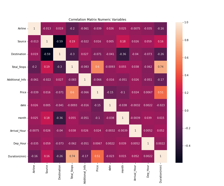
Figure 1. Heatmap of feature correlation (Figure credit: Original).

The next step is to draw line charts to observe the change trend of the above-mentioned several highly correlated features and prices. The relation of duration and price are demonstrated in Figure 2. Moreover, the relation of total stop and data are displayed in Figure 3. Although there is a strong correlation between travel time and price, the changing trend of the two is very twists and turns, and there is no obvious linear relationship. Contrary to the above is the relationship between the transfer station and the price. From the line chart, it can be clearly observed that the two are positively correlated linearly. The relationship between date and price is also in a state of continuous fluctuation, but from the general trend, the later the date of each month, the lower the air ticket price.

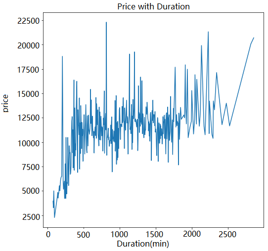
Figure 2. Relation of duration and price (Figure credit: Original).

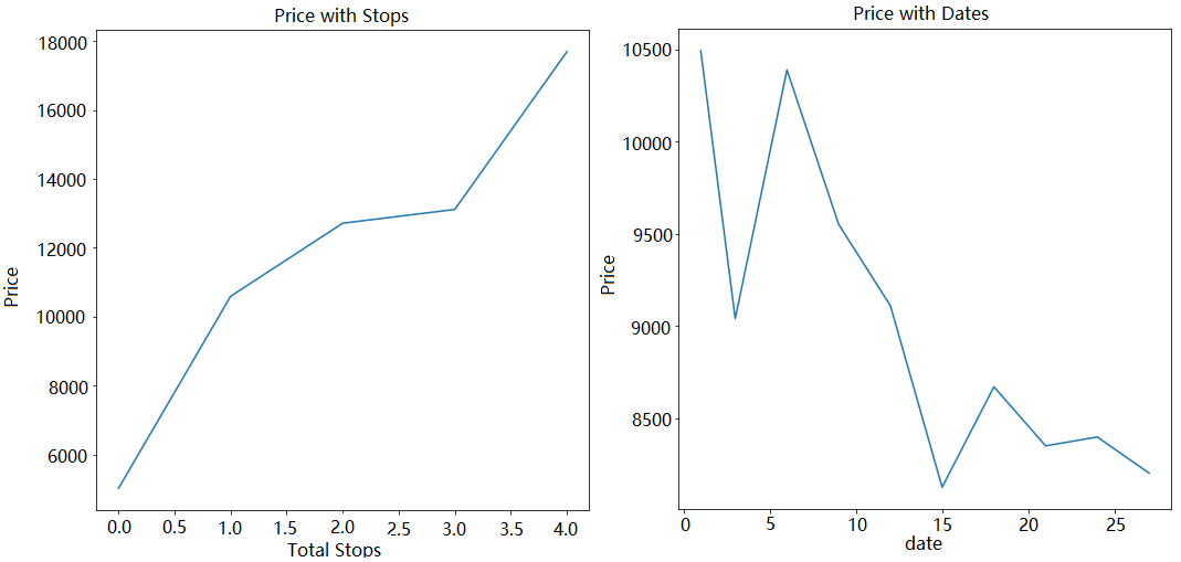
Figure 3. Relation between total stops and price (left), between date and price (right) (Figure credit: Original).

This section discusses how the trained model performs on the data in the test set. Here are the steps in detail. First, put the data in the data training set into the four models of ridge, random forest, XGB and K-Neighbors regression mentioned in section 2 for training, and use the trained model to predict the flight price for the data in the test set. The forecast outcomes of the four models are shown in Table 1.

Table 1. Result comparison of the four models.

R² has the highest score for XGB (0.89468), followed by Random Forest (0.83592). K-Neighbors and the first two models have a large score difference, ranking third with 0.64988. The lowest score is Ridge Regression, with only 0.45180, which even has a large difference with K-Neighbors.

The best RMSE scoring results and the lowest scoring results are XGB, Random Forest, K- Neighbors, and Ridge. The scoring of the model is consistent with the R² result.

The last evaluation index MAE is slightly different. The model with the best scoring result is Random Forest, followed by XGB. This index has the highest score for ridge regression, which is twice that of Random Forest. The score of K-Neighbors is slightly lower than that of ridge regression, but still higher, close to three times that of XGB.

4. Discussion

Summarizing the above three indicators, it can be seen that Random Forest regression and XGB regression, both of which belong to ensemble learning, have better prediction effects, that is, ensemble learning is more accurate than other types of regression model predictions, followed by K-Neighbors, and Ridge regression has the worst predictive ability. The reason for Ridge's poor performance may be that the design concept of ridge regression was originally designed to solve the problem of multicollinearity, but there is no significant correlation between the data variables used in this paper, and the model parameter alpha will not solve the prediction of this paper. In addition, the poor prediction results of K-Neighbors may also be caused by this reason. Then XGB regression based on gradient boosting tree and Random Forest regression based on random forest can better capture the complex relationship of dozens of variables in the data set by combining multiple weak learners. Through the comparison of the above indicators, compared with the traditional regression model, the regression model based on ensemble learning has reason to believe that it has a better ability to deal with regression problems.

5. Conclusion

This paper studies four regression prediction models for predicting flight prices, which belong to Random Forest regression and XGB regression of ensemble learning, Ridge regression and K-Neighbors based on the expansion of the least squares method. Use a grid search based on the model predictions to select the model parameters that give the best prediction results. Through the three evaluation indicators of R², RMSE and MAE, it can be found that the prediction results of the four methods are relatively obvious, XGB regression and Random Forest regression have the best prediction effects, which indicates ensemble learning is very suitable for regression prediction. While Ridge regression and K-Neighbors are not effective. In the training process, it can be found that the training set of K-Neighbors works well, but the effect on the test set is not good, and it is easy to overfit. This requires constant adjustment of the k value to lessen the complexity of the model. Ridge regression itself is not suitable for the low-correlation data sets used in this paper, so the use of this model for data set training can be avoided in the future use of low-correlation variable data sets. At the same time, this paper also has some limitations. In the parameter selection of K-Neighbors, a variety of choices about the value of k are provided, but the model prediction results still have obvious overfitting, which may be due to improper selection of parameters when grid search, only the best combination of parameters is pursued, resulting in a reduction in the model's ability to generalize given unfamiliar input while still using its best parameters. But in general, the research results of this paper select the optimal model for flight forecasting, which can help passengers choose more economical prices to improve passenger's budget planning. The optimal model can also provide reference for airlines to adjust pricing strategies, and help them attract more customers buy tickets.

References

[1]. Groves, W., & Gini, M. (2011). A regression model for predicting optimal purchase timing for airline tickets. 1-19.
[2]. Huang, H. C. (2013). A hybrid neural network prediction model of air ticket sales. Telkomnika Indonesian Journal of Electrical Engineering, 11(11), 6413-6419.
[3]. Janssen, T., Dijkstra, T., Abbas, S., & van Riel, A. C. (2014). A linear quantile mixed regression model for prediction of airline ticket prices. Radboud University, 3, 1-34.
[4]. Papadakis, M. (2014). Predicting Airfare Prices. Clerk Maxwell, 1-5.
[5]. Ren, R., Yang, Y., & Yuan, S. (2014). Prediction of airline ticket price. University of Stanford, 1-5.
[6]. Chen, Y., & Farias, V. F. (2018). Robust dynamic pricing with strategic customers. Mathematics of Operations Research, 43(4), 1119-1142.
[7]. Hoerl, A. E., & Kennard, R. W. (1970). Ridge regression: Biased estimation for nonorthogonal problems. Technometrics, 12(1), 55-67.
[8]. Zhou, X., Zhu, X., Dong, Z., & Guo, W. (2016). Estimation of biomass in wheat using random forest regression algorithm and remote sensing data. The Crop Journal, 4(3), 212-219.
[9]. Avanijaa, J. (2021). Prediction of house price using xgboost regression algorithm. Turkish Journal of Computer and Mathematics Education (TURCOMAT), 12(2), 2151-2155.
[10]. Alsayadi, H. A., Abdelhamid, A. A., El-Kenawy, E. S. M., Ibrahim, A., & Eid, M. M. (2022). Ensemble of Machine Learning Fusion Models for Breast Cancer Detection Based on the Regression Model. Fusion: Practice & Applications, 9(2) 19-26.
Cite this article
Liu,J. (2024). Feature correlation analysis and comparison of machine learning models for air ticket price prediction. Applied and Computational Engineering,30,271-278.
Data availability
The datasets used and/or analyzed during the current study will be available from the authors upon reasonable request.
Disclaimer/Publisher's Note
The statements, opinions and data contained in all publications are solely those of the individual author(s) and contributor(s) and not of EWA Publishing and/or the editor(s). EWA Publishing and/or the editor(s) disclaim responsibility for any injury to people or property resulting from any ideas, methods, instructions or products referred to in the content.
About volume
Volume title: Proceedings of the 2023 International Conference on Machine Learning and Automation
© 2024 by the author(s). Licensee EWA Publishing, Oxford, UK. This article is an open access article distributed under the terms and
conditions of the Creative Commons Attribution (CC BY) license. Authors who
publish this series agree to the following terms:
1. Authors retain copyright and grant the series right of first publication with the work simultaneously licensed under a Creative Commons
Attribution License that allows others to share the work with an acknowledgment of the work's authorship and initial publication in this
series.
2. Authors are able to enter into separate, additional contractual arrangements for the non-exclusive distribution of the series's published
version of the work (e.g., post it to an institutional repository or publish it in a book), with an acknowledgment of its initial
publication in this series.
3. Authors are permitted and encouraged to post their work online (e.g., in institutional repositories or on their website) prior to and
during the submission process, as it can lead to productive exchanges, as well as earlier and greater citation of published work (See
Open access policy for details).