1. Introduction

1.1. Problem background

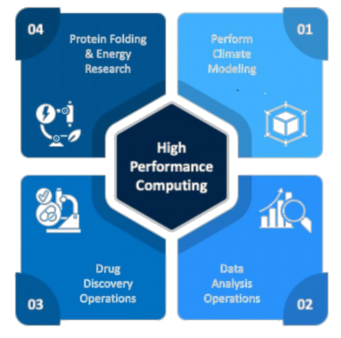
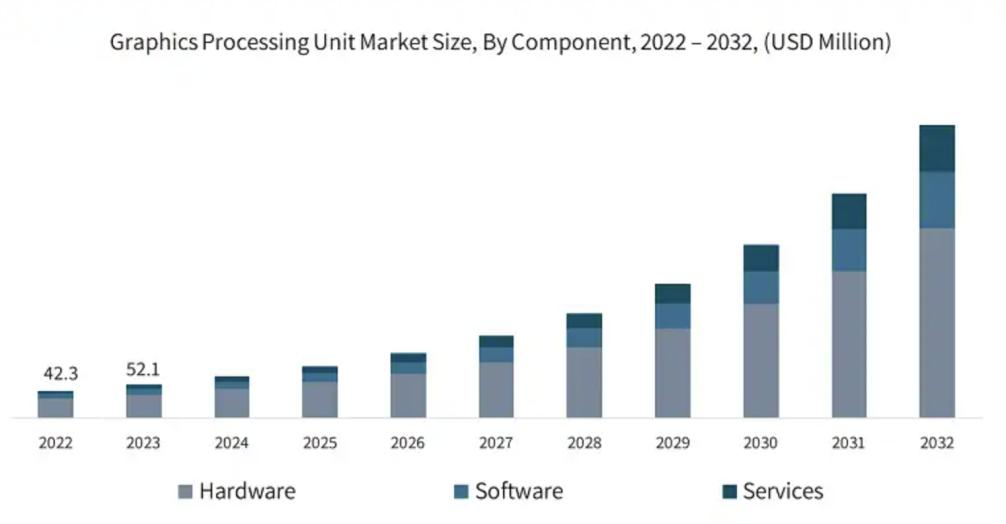
The demand for High-Performance Computing (HPC) has grown significantly across various fields, with the market size reaching approximately $5.002 billion in 2023 and projected to expand at a Compound Annual Growth Rate (CAGR) of over 7% in the coming years [1]. Despite the benefits HPC provides, it also poses notable environmental challenges. For example, the power consumption of supercomputers has approached or surpassed 50 megawatts, with annual energy consumption increasing at a rate of 20% to 40%. In 2020, the Information and Communication Technology (ICT) sector, which includes HPC, was responsible for an estimated 1.8% to 2.8% of Global Greenhouse Gas (GHG) emissions, a level comparable to that of the aviation industry (see Figure 1).

Simultaneously, the substantial rise in energy consumption and carbon emissions from HPC systems, coupled with the high-power demands of network architectures and water wastage in cooling systems, has raised significant environmental concerns. To address this, our team employ a mathematical model to assess the total carbon emissions resulting from HPC energy consumption, with the goal of formulating practical recommendations to mitigate its environmental impact.

1.2. Problem restate

The overarching goal of our team is to quantify the total carbon emissions resulting from HPC energy consumption and assess its environmental impact, while developing a practical set of recommendations to mitigate this impact. Specifically, our objectives are as follows.

1. Understand the problem: Model and estimate the global number of HPC devices and the energy consumption of individual HPC units. Consider the range of total annual energy consumption in global HPC centers under full load and average utilization rates [2].

2. Develop a model: Create a model to calculate the total carbon emissions and environmental impact of HPC energy consumption, taking into account energy production methods and varying energy mixes.

3. Apply the model: Utilize the model to explore the impact of HPC growth, increased energy demand from other sectors, and potential changes under different energy sources and combinations, with projections for 2030.

4. Expand the model: Extend the model to assess the effect of increasing renewable energy proportions in HPC energy consumption on carbon emissions reduction. Additionally, evaluate other critical environmental factors, such as water use and network architecture.

5. Share and advise: Share the model, conduct a sensitivity analysis, and draft a letter to the United Nations Advisory Committee, recommending the incorporation of HPC’s environmental impact into the 2030 development goals, using our findings and recommendations to support this proposal.

1.3. Our work

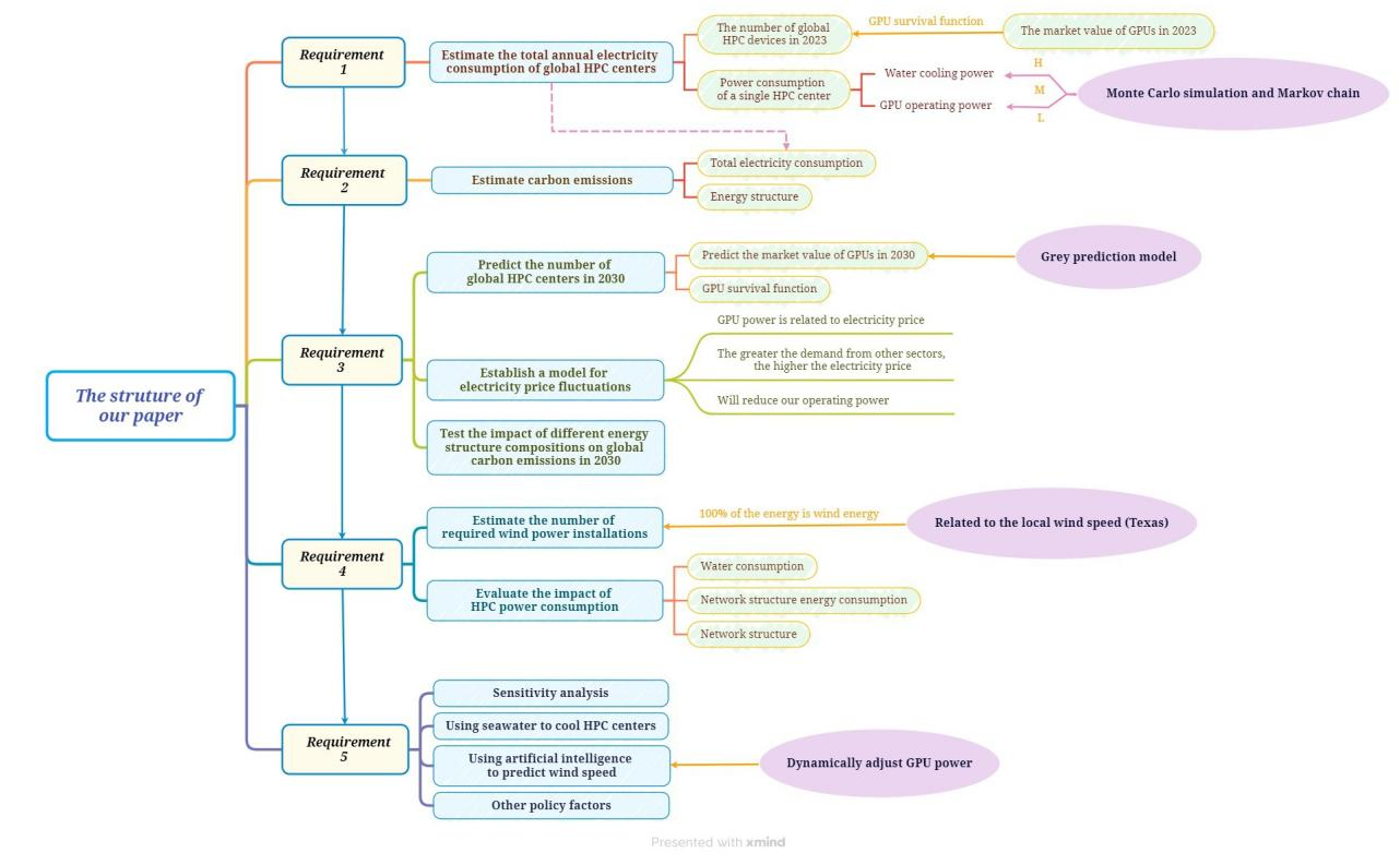
As shown in Figure 2, our work could be divided into 5 parts.

(1) The first part involves understanding the problem. We estimated the number of HPC devices worldwide in 2023 based on the GPU market capitalization for that year. At this stage, we applied the GPU survival function, which predicts the expected lifespan of a GPU and calculates the probability that the GPU will not fail within a specific period. We then used Monte Carlo simulations and Markov chains to estimate the power consumption of a single HPC center under full load, low load, and average load conditions, accounting for both water for cooling and GPU operating power. This allowed us to calculate the total annual power consumption of HPC centers globally.

(2) The second part focuses on model creation. We used carbon emission factors, energy structure data, and the total electricity consumption calculated in the first framework to estimate the carbon emissions.

(3) The third part involves applying the model. First, we used a gray prediction model to forecast the market value of GPUs in 2030. The number of global HPC centers in

2030 was then determined by combining the predicted GPU market value with the GPU survival function from the first framework. We also established an electricity price fluctuation model, where GPU power consumption is linked to electricity prices. As demand from other sectors increases, electricity prices rise, which in turn reduces GPU efficiency.

(4) The fourth part expands the model by increasing the proportion of renewable energy (specifical wind energy) in the energy mix to 100%, in order to assess its impact on reducing carbon emissions. Additionally, we considered critical environmental factors such as water use and network architecture to evaluate the impact of HPC power consumption.

(5) Lastly, we conducted a sensitivity analysis on the model, incorporating seawater cooling for HPC centers and using artificial intelligence to predict wind speeds for dynamically adjusting GPU power. We also considered other policy factors to refine the model further.

Our paper consists of five sequential parts. first, we estimated global HPC device numbers in 2023, using GPU market data, survival functions, and simulations to calculate power consumption. Second, we created a model to estimate carbon emissions based on energy use. Third, we forecast the 2030 GPU market, predicted HPC center numbers, and linked power consumption to electricity price fluctuations. Fourth, we expanded the model to assess the impact of 100% renewable energy and environmental factors. Finally, we refined the model with sensitivity analysis, incorporating seawater cooling, AI wind speed predictions, and policy factors.

2. Assumptions and justifications

Assumption 1: The power of GPUs within the same server is identical.

Justification: The same server is solving the same task, so the power consumption is basically the same.

Assumption 2: When the server is working, all electrical energy is converted into heat energy and absorbed by water.

Justification: According to the law of conservation of energy, the electrical energy consumed by the server is converted into heat energy and absorbed by the cooling system's water. This ensures that the server's temperature remains within a safe range.

Assumption 3: The lifespan of a single GPU is assumed to follow a normal distribution with a mean of 3 and a standard deviation of 1.5, with a maximum lifespan of 10 years.

Justification: This means that most GPUs will have a lifespan close to the mean of 3 years, but there will be some variation. Additionally, a maximum lifespan of 10 years is set for each GPU.

Assumption 4: The transitions of different power consumption of the server are assumed to follow a Markov chain process, where the system or state has no memory.

Justification: This means that the power consumption transitions of the server follow a Markov chain process, where the system's current state transition depends only on the current state and not on the previous states. This property is also known as "Markovian" or "memorylessness."

Assumption 5: During the water-cooling process of the server, the temperature and flow rate of the water are assumed to be constant.

Justification: When using Monte Carlo simulations and Markov chain modeling to estimate the power consumption of a single HPC center, it is assumed that the temperature and flow rate of the water in the server's cooling process remain unchanged

3. Notations

Table 1, titled "Symbols and Units of Used Parameters (Partial)", provides a list of key parameters along with their corresponding symbols and units. 

4. Global HPC equipment power calculation model

Basic Process Brief. The development of the global HPC equipment power calculation model involves three key components: assessing the global number of HPC devices, calculating the power consumption of each device, and simulating changes in power consumption over time. The model must account for factors such as the global distribution of HPC devices, the power consumption of GPUs under varying load conditions, and the sources of power used. The following outlines the detailed steps:

4.1. Forecast of global HPC

4.1.1. GPU survival model

To estimate the number of global HPC devices, we begin with the fundamental computing unit of HPC—the GPU. By analyzing the market value of GPUs, we can infer the total number of global HPC devices. Let  $$ V\left(t\right)$$  represent the market value of GPUs at time  $$ t$$ , and let  $$ P\left(t\right)$$  denote the unit price of a single GPU [3]. The number of GPUs,  $$ N\left(t\right)$$ , for a given year  $$ t$$  can then be expressed as:

$$ \begin{array}{c}Nt=\frac{Vt}{Pt}\end{array}$$(1)

However, GPUs have a finite service life, and newly added GPUs will remain in use in subsequent years. We assume that the survival function of GPUs follows a normal distribution with a mean of 3 years and a standard deviation of 1.5 years, with a maximum service life of 10 years. The survival function 

$$ S\left(t\right)$$  can be expressed as follow, where  $$ \varnothing $$  is the Cumulative Distribution Function (CDF) of the standard normal distribution,  $$ \mu $$  is the mean,  $$ \sigma $$  is the standard deviation,  $$ L_{max}$$  is the maximum limit for  $$ t$$ .

where  $$ \mu $$  is the mean and  $$ \sigma $$  is the standard deviation. Using this survival function, we can estimate the number of GPUs in global HPC devices each year with the following equation, where  $$ Tt$$  is the total amount of time:

$$ \begin{array}{c}N=M+\sum _{i=0}^{r-1}M\times S (r-1)\end{array}$$(2)

$$ \begin{array}{c}Dt=Tt-1-\sum _{i=0}^{t-1}Ni\times S\left(t-i\right)\end{array}$$(3)

4.1.2. Global HPC quantity

By plotting a time series of the number of GPUs each year, we can analyze the changes in the global HPC device population. This chart illustrates the growth trend and patterns in the number of HPC devices worldwide, as shown in Figure 3.

4.2. Power estimation based on Markov chains and monte carlo simulation

To estimate the annual power consumption of HPC devices worldwide, we first calculate the power consumption of a single HPC device under three scenarios: the HPC equipment operates at high load throughout the year; the HPC equipment fluctuates between high, medium, and low loads during the year, and the HPC equipment operates at low load throughout the year. These scenarios allow us to estimate the dynamic range of electricity consumption. The table below presents the power consumption ranges for high, medium, and low load conditions [4].

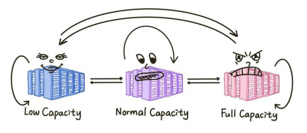
Figure 4 illustrates a Markov chain model depicting the state transitions of a High-Performance Computing (HPC) system under varying capacity levels. The system comprises three states: Low Capacity, Normal Capacity, and Full Capacity, each representing different workload conditions. The arrows represent the possible transitions between these states, indicating how the system can either shift to another state or remain in the same state. These transitions are governed by fixed probabilities, which depend on workload fluctuations. This model provides insights into the system's behavior over time and can inform resource management strategies to optimize performance.

4.2.1. High load power consumption calculation

The primary power sources for our HPC system are divided into two components: the working power of the HPC equipment itself and the power required for water cooling. We assume that 100% of the electrical energy consumed by the HPC system is converted into heat and absorbed by the water-cooling system. This is because the power required by the cooling tower is equivalent to the working power of the HPC system. Assuming that the working power of HPC at time  $$ t$$  is  $$ P\left(t\right)$$, the energy consumed by HPC in a period of one year (365 days, 24 hours a day) is as follows:

$$ \begin{array}{c}\sum _{t=1}^{365}Pt*24\end{array}$$(4)

In high load situations, we assume that the power consumption of all GPUs is uniformly distributed between 350W and 375W. Monte Carlo simulation, a technique used to model the probability of various outcomes in processes influenced by random variables, is employed to calculate the power consumption of global HPC devices under high load. Using Python's built-in random function, we sample the daily GPU power consumption from the specified uniform distribution to determine the daily working power $$ Pt $$ .

4.2.2. Low load power consumption calculation

In low load situations, we assume that the power consumption of all GPUs is uniformly distributed between 150W and 250W. Using Monte Carlo simulation, we calculate the power consumption of global HPC devices under low load.

4.2.3. Average high load power consumption calculation

HPC devices do not remain in a constant state of high or low load; instead, they fluctuate dynamically between these states. This behavior can be modeled using a Markov chain. In this Markov chain representation of HPC, there are three states: full load, normal load, and low load, with transitions between these states. The state transition matrix 

$$ P$$  can be expressed as:

4.2.4. HPC power consumption calculation results

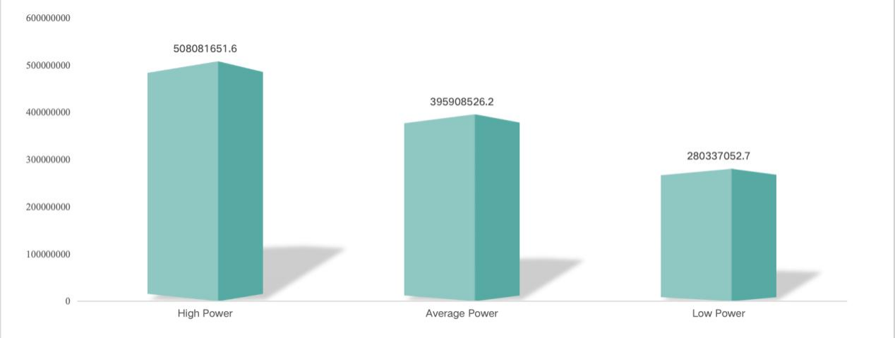
The diagram illustrates the amount of energy use over the range of high power, low power and average power. This result is used to evaluate and determine the amount of heat absorbed by the water-cooling system, as shown in Figure 5.

5. Global HPC equipment carbon emission estimation model and future prediction model

5.1. GPU market value prediction based on grey prediction model

5.1.1. Gray prediction principle

The gray prediction model GM (1, 1) is a forecasting method designed for systems with uncertain factors, particularly useful for predicting data series with incomplete information [4]. The basic principle involves generating a regular data series, constructing a differential equation model, and estimating the model parameters using the least squares method to predict system behavior. The core of gray prediction is to apply a cumulative generation (1-AGO) process to the original data series, creating a new series that reveals a clear upward or downward trend, which is then used to build a first-order linear differential equation model for forecasting.

In this paper, we use the enhanced GM (1, 1) model with other influencing factors to predict STT [5]. We define  $$ X^{\left(0\right)}$$  as the original data sequence of STT from 1980 to 2020:

$$ \begin{array}{c}{X}^{\left(0\right)}=\{X_1^0,X_2^0,X_3^0,\cdots X_n^0\}\end{array}$$(5)

And then we get the whitened equation:

$$ \frac{d{X}^{\left(1\right)}}{dt}+a{X}^{\left(1\right)}-b$$

where,  $$ X^{\left(1\right)}$$  is the cumulative generating operation sequence of  $$ X^{\left(0\right)}$$ . Then we use the least square method (OLS) to obtain parameters  $$ a$$  and  $$ b$$  as：

$$ \begin{array}{c}\widehat{a}=(B^{T}B{)}^{-1}{B}^{T}Y\end{array}$$(7)

Where

$$ \begin{array}{c}B=\left[\begin{array}{cc}-z_2^{\left(1\right)}& 1\\ -z_3^{\left(1\right)}& 1\\ \dots & \dots \\ -z_n^{\left(1\right)}& 1\end{array}\right] Y=\left[\begin{array}{c}{X}_2^{\left(0\right)}\\ X_3^{\left(0\right)}\\ \dots \\ X_n^{\left(0\right)}\end{array}\right]\end{array}$$(8)

$$ \begin{array}{c}{z}_k^1=0.5(X_k^1+X_{k-1}^1\end{array}$$(9)

The respective time response sequence of the model is:

$$ \begin{array}{c}{\widehat{x}}_{k+1}^{ 1 }=\left(X^{\left(0\right)}\left(1\right) -\frac{b}{a}\right)e^{-\underset{\_}{ak}}+\frac{b}{a} k= \mathrm{1,2},3,\dots ,n-1\end{array}$$(10)

$$ \begin{array}{c}{\widehat{x}}_k^0={\widehat{x}}_k^1-{\widehat{x}}_{k-1}^1\end{array}$$(11)

To test the model, we define the gray prediction subsequence as:

$$ \begin{array}{c}\stackrel{\left(0\right)}{\hat{X}}=\{{\underset{1}{\hat{X}}}^{0_1},{\underset{2}{\hat{X}}}^{0_1},{\underset{3}{\hat{X}}}^0...{\underset{n}{\hat{X}}}^{0_n}\}\end{array}$$(12)

Residuals can be obtained:

$$ \begin{array}{c}{e}_k=x_k^0-{\xi }_k^0,k=\mathrm{1,2},\dots ,n\end{array}$$(13)

Calculate the variance  $$ S_1$$  of the original sequence  $$ x^0$$  and the variance  $$ S_2$$  of the residual  $$ e$$.

$$ \begin{array}{c}{S}_1=\frac{1}{n}{\sum _{k=1}^n\left(x_k^0-\overline{x}\right)}^2 \end{array}$$(14)

$$ \begin{array}{c} S_2=\frac{1}{n}{\sum _{k=1}^n\left(e_k^0-\overline{e}\right)}^2\end{array}$$(15)

Finally, the test error ratio of  $$ S_1$$  and  $$ \mathrm{ }{\mathrm{S}}_2$$  is calculated.

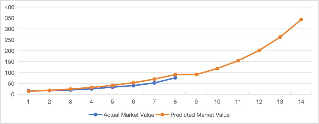
5.1.2. Analysis of gray prediction results

The result analysis of gray prediction primarily involves evaluating the accuracy of the model and obtaining the predicted values. By comparing the predicted values with the actual values and calculating the residual and relative errors, the prediction accuracy of the model can be assessed. The forecast results typically provide the number of HPC devices for different years, offering insights into the future development trends of the HPC market. Figure 6 blow are the results from the gray prediction.

5.2. Carbon emission estimation of HPC equipment

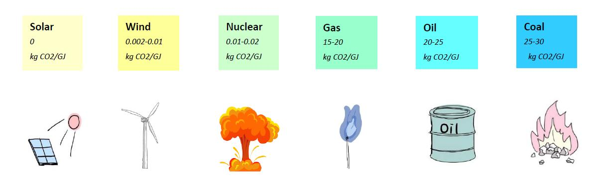
5.2.1. Design different energy structures

When estimating the carbon emissions of HPC equipment, it is essential to consider various energy structures. The energy mix design involves determining the proportion and use of different energy sources, such as coal, oil, natural gas, and non-fossil energy. These energy sources have distinct carbon emission factors, which directly influence the total carbon emissions [6], as shown in Figure 7.

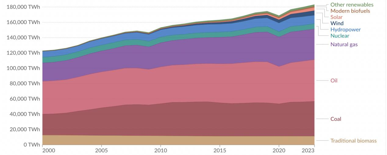
5.2.2. Impacts of carbon emissions from different energy structures

Different energy structures have a substantial impact on the carbon emissions of HPC equipment. For instance, coal produces significantly higher carbon emissions as an energy source compared to natural gas and non-fossil energy sources. Therefore, optimizing the energy mix and increasing the share of clean energy is crucial for reducing the carbon emissions of HPC equipment, as shown in Figure 8.

5.3. Future GPU power prediction

Based on the Markov chain prediction model, we can forecast future GPU power consumption. AMarkov chain is a stochastic process in which the future state depends solely on the current state, not on past states. In GPU power prediction, the Markov chain is used to simulate the transition probabilities between different power states, enabling the prediction of future power consumption. By combining this with the number of GPUs obtained from the previous gray prediction, we can further estimate the total power consumption [7].

5.4. Electricity price fluctuation model

Electricity price fluctuations significantly impact the operating power of GPUs. Changes in electricity prices can alter the GPU's operating state as it adjusts to shifts in electricity costs. The electricity price fluctuation model can predict these price trends and quantify their effect on GPU power consumption using relevant formulas. For instance, an increase in electricity prices may prompt GPUs to reduce workload in order to conserve energy, while a decrease in electricity prices may encourage higher workload to capitalize on lower-cost power. Constructing the electricity price fluctuation model typically involves time series analysis, such as the ARMA model, while considering factors like market supply and demand, policy changes, and other relevant variables.

6. HPC equipment environmental factor assessment and 100% energy challenge

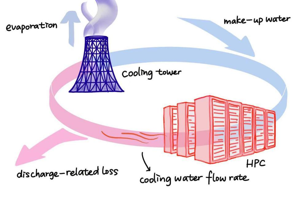
6.1. Water calculation

In High-Performance Computing (HPC) systems, water consumption primarily arises from the cooling system. As HPC equipment generates substantial heat during operation, a cooling system is essential to maintain the optimal operating temperature. These systems typically include water-cooled radiators and coolant circulation systems, both of which require water to absorb and transfer heat. The water consumption can be estimated using the following formula:

$$ \begin{array}{c} W=F\times T\end{array}$$(16)

where  $$ W$$  is water consumption,  $$ F$$  is the cooling system flow, and  $$ T$$  is the operation time.

The flow rate of the cooling system refers to the volume of water passing through the system per unit of time, while the operating time denotes the actual runtime of the HPC equipment. This calculation can serve as a reference for effective water resource management in HPC systems.

6.2. Network structure power calculation

One common network architecture used in HPC systems is the Fat Tree topology. This architecture consists of three types of switches: edge switches, aggregation switches, and core switches. The primary source of power for these switches comes from their own power supplies, as well as the devices to which they are connected. Electricity consumption can be calculated using the following formula:

$$ \begin{array}{c}Total Power Consumption=N_{edge}\times P_{edge}+N_{agg}\times P_{agg}+N_{core}\times P_{core}\end{array}$$(17)

where  $$ N_{edge}$$  is the number of edge switches,  $$ P_{edge}$$  is the power consumption of each edge switch;  $$ N_{agg}$$  is the number of aggregation switches,  $$ P_{agg}$$  is the power consumption of each aggregation switch;  $$ N_{core}$$  is the number of core switches,  $$ P_{core}$$  is the power consumption of each core switch.

Figure 9 visualizes the network topology diagram of Fat Tree network architecture for a more intuitive understanding.

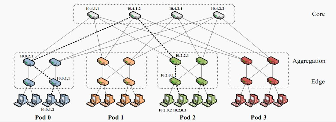
The formula for calculating the number of switches depends on the specific network size and design requirements. For example, each pod consists of  $$ (k/2)2$$  servers & 2 layers of  $$ k/2$$  k-port switches, each edge switch connects to  $$ k/2$$  servers &  $$ k/2$$  aggregation switches, each aggregation switch connects to  $$ k/2$$  edge &  $$ k/2$$  core switches,  $$ (k/2)2$$  core switches: each connects to k pods

6.3. 100% energy challenges

Considering the challenges posed by 100% wind energy, we focus on the impact of the instability and unpredictability of wind energy on the operation of HPC equipment [8]. The formula for calculating wind energy can be expressed as:

$$ \begin{array}{c}E\left(v\right)=\{\begin{array}{cc}0,& v<v_{min}\\ 0.5\times A\times \rho \times v^3,& v_{min}\le v\le v_{max}\\ 0,& v>v_{max}\\ & \end{array} \end{array}$$(18)

where  $$ E$$  stands for wind energy,  $$ \rho $$  stands for air density, A stands for wind area, and  $$ v$$  stands for wind speed. To ensure the proper operation of the HPC device's GPU during the state transition process described by the Markov chain, it is necessary to evaluate the stability and reliability of wind energy using the time series diagram of local wind speed. The formula for the state transition probability of the Markov chain is, where  $$ p_{ii}\left(n\right)$$  represents the n-step transition probability from state  $$ i$$  to state  $$ j$$:

$$ \begin{array}{c}{p}_{ii}\left(n\right)=P\{x_{m+n}=j \backslash x_m=i\}\end{array}$$(19)

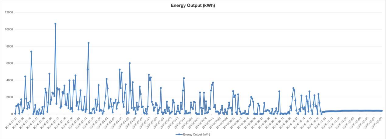
As shown in Figure 10, the diagram illustrates the time series variations of local wind speed over different periods, used to evaluate the stability and reliability of wind energy to ensure the normal operation of the HPC device's GPU.

In order to maintain the normal operation of the GPU, we need to set up enough wind equipment to ensure that the wind speed is low enough to provide enough energy. Assuming that the maximum output power of the wind device is  $$ P_{max}$$, then according to the wind speed and the efficiency of the wind device, we can determine the maximum wind device setting as:

$$ \begin{array}{c}{P}_{max}=F_{required}÷n\end{array}$$(20)

Where  $$ E_{required}$$  is the minimum energy required for the GPU to operate and  $$ \eta $$  is the conversion efficiency of the wind device. In this way, we can ensure that HPC equipment receives an adequate energy supply even at low wind speeds.

7. Establishment and countermeasures

7.1. Utilizing artificial intelligence for dynamic GPU power adjustment

A study by the National Renewable Energy Laboratory highlights the potential of AI and machine learning to improve energy efficiency in renewable energy systems, such as wind farms. Similarly, applying AI to adjust GPU workloads based on wind availability can reduce the need for additional wind turbines [9].

To implement this approach, our group selected the Long Short-Term Memory (LSTM) model for predicting wind speeds. The LSTM model, a type of Recurrent Neural Network (RNN), is particularly well-suited for time-series forecasting due to its ability to learn long-term dependencies in sequential data. Figure 11 is the basic architecture of the LSTM model.

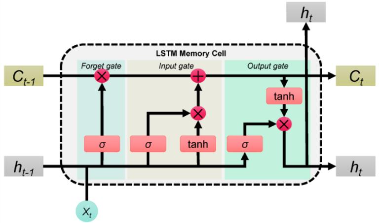
The input gate in LSTM regulates how much of the current input information is allowed to impact the present state. The mathematical formulation for the input gate is:

$$ \begin{array}{c}{i}_t=\sigma (W_i\cdot [h_{t-1},x_t]+b_i)\end{array}$$(21)

where  $$ i_t$$  is the input gate,  $$ \sigma $$  is the ReLU function,  $$ W_i$$  is the weight matrix, [ $$ ht-1, xt$$ ] is the concatenation of the previous hidden state and the current input, and  $$ b_i$$  is the bias.

The forget gate determines the degree to which the previous state is maintained.

The mathematical expression is:

$$ \begin{array}{c}{f}_t=\sigma (W_f\cdot [h_{t-1},x_t\left]\right)+b_f\end{array}$$(22)

where  $$ f_t$$  is the forget gate.

The output gate determines how the current state influences the output at the next moment. The mathematical expression for the output gate is:

$$ \begin{array}{c}\underset{t}{\tilde{\mathcal{C}}}=\tanh (W_c\cdot [h_{t-1},x_t]+b_c)\end{array}$$(23)

$$ \begin{array}{c}{C}_t=f_t\cdot C_{t-1}+i_t\cdot \underset{t}{\tilde{C}}\end{array}$$(24)

where  $$ \underset{}{\tilde{\mathcal{C}}}$$ t is the candidate memory unit state.

The hidden state is updated using the output gate and the current memory cell state, with the update formula being:

$$ \begin{array}{c}{h}_t=o_t\cdot \tanh (C_t)\end{array}$$(25)

We initialize the learning rate of the STFN at 0.001, train the model over 50 epochs, and utilize the Adam optimizer for network optimization. To adjust the learning rate, we apply the cosine annealing scheduler.

$$ \begin{array}{c}l{r}_t=l{r}_{min}+0.5(l{r}_{max}-l{r}_{min})(1+\mathit{cos}(\frac{T_{cur}}{T_{max}}\pi ))\end{array}$$(26)

where  $$ l{r}_t$$  is the current learning rate,  $$ l{r}_{\mathrm{m}\mathrm{i}\mathrm{n}}$$  and  $$ l{r}_{\mathrm{m}\mathrm{a}\mathrm{x}}$$  are the minimum and maximum learning rates,  $$ T_{cur}$$  is the current epoch, and  $$ T_{\mathrm{m}\mathrm{a}\mathrm{x}}$$  is the maximum epoch. We use the MSE loss function to train our model.

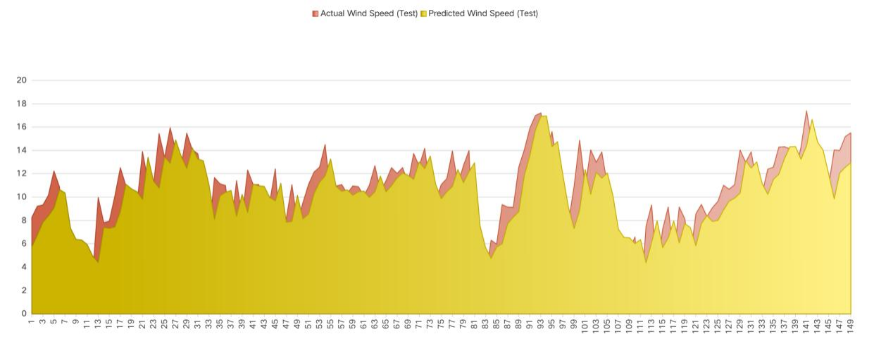
Wind turbines often face underutilization during periods of low wind speed, resulting in inefficiencies in energy production. However, AI-driven algorithms can effectively align GPU workload demands with periods of high wind availability. For example, when high wind speeds are forecasted, AI can schedule GPUs to operate at full capacity, optimizing energy utilization. Conversely, during low wind speed periods, GPUs can function at reduced power levels, minimizing energy wastage. This approach not only enhances the usage of renewable energy but also decreases reliance on traditional, carbon-intensive energy sources. Figure 12 is the LSTM Wind Speed Forecasting Results.

7.2. Use of seawater for cooling

(1) As our investments progress, we have determined that using deep-sea water for High-Performance Computing (HPC) cooling will be the most effective strategy moving forward. Currently, the environmental impact of various cooling technologies—such as water cooling, liquid cooling, and air cooling—remains a topic of intense debate. Water cooling, for instance, faces challenges such as leakage risks and high water consumption. Coolant-based cooling systems require specialized, expensive coolants, which pose a significant environmental pollution risk. Air cooling, while common, is less effective for high-performance systems, generating high noise levels due to the powerful fans required [10].

In light of these challenges and considering future advancements in scientific research, we propose a solution: placing HPC systems in deep-sea water regions. Using seawater for cooling offers several advantages, primarily due to its favorable physical properties. The temperature of deep seawater typically ranges from 2°C to 4°C, significantly lower than the typical circulating water temperatures of 10°C to 15°C found in traditional cooling systems. This substantial temperature difference allows seawater to dissipate heat more effectively, reducing the energy required to maintain optimal system performance. Figure 13 below is a simple diagram illustrating the principle of this cooling process:

Second, seawater has a slightly lower specific heat capacity, approximately 3850  $$ J/(kg·K)$$ , compared to freshwater, which has a specific heat capacity of around 4182  $$ J/(kg·K)$$ . This difference allows seawater to absorb heat more rapidly, making it an ideal cooling medium. Additionally, the reduced evaporation rate during heat absorption is a key advantage, as seawater requires less energy to remove the same amount of heat. With a latent heat of vaporization of about 2260  $$ kJ/kg$$ , seawater minimizes water loss while maximizing cooling efficiency, making it a resource- efficient and environmentally friendly option.

In fact, Microsoft began researching underwater data centers in 2013. In their trials, only six out of 855 servers failed, compared to eight out of 135 servers on land. This demonstrates the effectiveness of underwater data centers in reducing failure rates. With continued advancements, it is expected that issues related to HPC cooling and environmental impact will be significantly improved in the future.

8. Model evaluation and further discussion

8.1. Strengths

This paper employs Monte Carlo simulation and gray prediction models for analysis. Monte Carlo simulation is a widely used statistical model that relies on random sampling techniques. Due to its use of random sampling, it can effectively quantify uncertainties and handle complex systems by considering multiple influencing factors. As a result, it is a highly flexible model. The gray prediction model, another established statistical method, is characterized by its simple formula and straightforward calculation. It is applicable to a broad range of data types and reduces the impact of random factors through the process of cumulative summation.

8.2. Weaknesses

The model used in this paper also has certain limitations. Monte Carlo simulation is highly sensitive to the randomly selected data, which can result in unstable solutions. On the other hand, the gray prediction model has a relatively rigid structure and tends to exhibit lower accuracy in long-term predictions.

8.3. Further discussion

In this paper, both models exhibit unstable solutions. For this problem, the model can be applied multiple times to each data set, and the average of the obtained solutions can be taken as the final result. This approach can help to stabilize the solution.

9. Conclusion

First, we estimated global GPU numbers through market value analysis, considering both new and legacy GPUs. Using GPU survival functions, we estimated the total number of GPUs worldwide in 2024 to be  $$ 1. 19\times 108$$ . By modeling GPU load states using a Markov transition process and Monte Carlo simulations, we calculated the average global HPC power consumption in 2024 to be  $$ 3.96\times 1011 kWh$$ , with maximum and minimum consumption at  $$ 5.08\times 1011 kWh$$  and  $$ 2.80\times 1011 kWh$$ . Combining carbon emission factors, maximum CO2 emissions reach  $$ 1.01\times 1014 kg$$  with power generation comprising 40% coal, 30% natural gas, 20% oil, and 10% renewable energy.

Using a gray prediction model, we projected 2030 GPU numbers to reach  $$ 5.67\times 108$$  units, with power consumption of  $$ 2.81\times 1012 kWh$$ . Our power fluctuation model suggests a potential 16% reduction in consumption due to rising electricity prices. Analysis of Szeged wind data showed that a single wind power unit produces maximum 23,230 kWh daily, requiring 47 units for 10,000 HPC nodes, though experiencing six zero-generation days annually.

Our water cooling tower model revealed annual water loss of  $$ 4.12\times 107 L$$  per HPC device. For a 10000-node HPC system using Fat Tree architecture, annual network energy consumption reaches  $$ 9.85\times 106 kWh$$ .

We propose two optimizations: an AI-based wind speed prediction model using LSTM ( $$ R2=0.7832$$ , outperforming random forest's 0.2028), and a seawater cooling solution potentially reducing evaporation losses by  $$ 1.18\times 107 L$$  annually.

References

[1]. Price, D. C., Clark, M. A., Barsdell, B. R., Babich, R., & Greenhill, L. J. (2016). Optimizing performance per watt on GPUs in high performance computing: Temperature, frequency and voltage effects.Computer Science - Research and Development, 31(3), 185–193. https: //doi.org/10.1007/s00450-016-0324-7
[2]. He, W., Ding, S., Zhang, J., Pei, C., Zhang, Z., Wang, Y., & Li, H. (2021). Performance optimization of server water cooling system based on minimum energy consumption analysis.Applied Energy, 303, Article 117620. https: //doi.org/10.1016/j.apenergy.2021.117620
[3]. Mugaishudeen, G., Manikandan, A. S. P., & Kannan, T. R. (2013). Experimental study of triple effect forced circulation evaporator at Perundurai Common Effluent Treatment Plant. J. Acad. Indus. Res., 1(12), May 2013. https: //www.researchgate.net/publication/316545200_Experimental_study_of_ Triple_Effect_Forced_Circulation_Evaporator_at_Perundurai_Common_Efflu ent_Treatment_Plant/figures?lo=1
[4]. Global Market Insights. (2024). High performance computing market size - By component (solutions, services), by deployment (cloud, on-premises), by organization size (small and medium-sized enterprise, large enterprise), by computation type, by application, by end-use & forecast, 2024–2032. https: //www.gminsights.com/industry-analysis/high-performance-computing- market
[5]. TechTarget. (2021). A comprehensive guide to HPC in the data center. https: //www.techtarget.com/searchdatacenter/tip/Top- considerations-for-HPC-infrastructure-in-the-data-center
[6]. Markets and Markets. (2022). High performance computing market industry report, size, share, global. Retrieved from https: //www.marketsandmarkets.com/Market-Reports/Quantum-High- Performance-Computing-Market-631.html
[7]. Rescale. (2015). The real cost of high performance computing. https: //rescale.com/blog/the-real-cost-of-high-performance-computing/
[8]. Cushman & Wakefield. (2023). Asia Pacific data centre construction cost guide 2023/2024. https: //www.cushmanwakefield.com/en/insights/apac-data-centre- construction-cost-guide
[9]. Li, B., Basu Roy, R., Wang, D., Samsi, S., Gadepally, V., & Tiwari, D. (2023). Toward sustainable HPC: Carbon footprint estimation and environmental implications of HPC systems. SC '23: Proceedings of the International Conference for High Performance Computing, Networking, Storage and Analysis, Article No. 19, 1–15. https: //doi.org/10.1145/3581784.3607035
[10]. Ritchie, H., & Roser, M. (2024). Energy production and consumption.Our World in Data.https: //ourworldindata.org/energy-production- consumption
Cite this article
Wang,H.;Su,Y.;Guo,Y. (2025). The environmental challenge of HPC: finding green power and cooling solutions for supercomputers. Advances in Engineering Innovation,16(6),21-34.
Data availability
The datasets used and/or analyzed during the current study will be available from the authors upon reasonable request.
Disclaimer/Publisher's Note
The statements, opinions and data contained in all publications are solely those of the individual author(s) and contributor(s) and not of EWA Publishing and/or the editor(s). EWA Publishing and/or the editor(s) disclaim responsibility for any injury to people or property resulting from any ideas, methods, instructions or products referred to in the content.
About volume
Journal:Advances in Engineering Innovation
© 2024 by the author(s). Licensee EWA Publishing, Oxford, UK. This article is an open access article distributed under the terms and
conditions of the Creative Commons Attribution (CC BY) license. Authors who
publish this series agree to the following terms:
1. Authors retain copyright and grant the series right of first publication with the work simultaneously licensed under a Creative Commons
Attribution License that allows others to share the work with an acknowledgment of the work's authorship and initial publication in this
series.
2. Authors are able to enter into separate, additional contractual arrangements for the non-exclusive distribution of the series's published
version of the work (e.g., post it to an institutional repository or publish it in a book), with an acknowledgment of its initial
publication in this series.
3. Authors are permitted and encouraged to post their work online (e.g., in institutional repositories or on their website) prior to and
during the submission process, as it can lead to productive exchanges, as well as earlier and greater citation of published work (See
Open access policy for details).