1. Introduction

Vegetable commodities are essential food items in people’s daily lives, and the price and availability of vegetables have a significant impact on people’s health and quality of life. In fresh supermarkets, the shelf life of vegetable commodities is generally short, and the quality deteriorates as the sales time increases. Most varieties, if not sold on the day, cannot be sold the next day. Due to the wide variety of vegetables sold in supermarkets and their diverse origins, vegetable procurement transactions usually take place between 3:00-4:00 in the morning. Therefore, businesses need to make replenishment decisions for various vegetable categories on the day without knowing the specific items and procurement prices, but understanding the historical sales and demand situations of each commodity. In traditional vegetable sales, pricing and replenishment decisions are usually made manually, which has some problems. Firstly, manual pricing and replenishment decisions are susceptible to human factors such as subjective consciousness, experience, and emotions. Secondly, manual pricing and replenishment decisions require a considerable amount of time and effort, and often fail to timely reflect market changes and demand fluctuations. Therefore, we need to adopt automated methods for pricing and replenishment decisions of vegetable commodities to improve efficiency, reduce errors, lower costs, and make decisions more objective and scientific.

2. Problem analysis

Analyzing the distribution patterns and relationships of sales volumes among different categories and individual items of vegetables. Utilizing the new data obtained through data preprocessing, due to the large volume of data, we discuss based on the time dimension: month. Scatter plots are drawn between different categories or individual items for analysis of distribution patterns. Regarding the relationships, which belong to evaluation models, we apply correlation analysis. Firstly, the relationship between sales volumes of six categories of vegetables is analyzed using the K-S test to determine that the data follows a normal distribution with a P-value > 0.05, and Spearman correlation coefficient is used to analyze the relationship between vegetable categories and sales volumes. For the relationship between the sales volumes of 251 individual vegetable items, cluster analysis can be used for classification, and then their relationships can be determined.

Based on the above, data after preprocessing is obtained. Replenishment plans are required to be made by category, analyzing the relationship between the total sales volume of each vegetable category and cost-plus pricing, and fitting using XG Boost and linear regression models. Based on historical sales data, the daily replenishment total for each vegetable category within the next week is predicted. Predictive models and time series analysis are employed. Meanwhile, for pricing strategies, the XG Boost algorithm is utilized to provide reasonable pricing strategies. Based on the optimal solution, replenishment plans and pricing strategies for the next week are formulated to ensure the maximization of sales revenue objectives.

3. Assumptions of the model

We assume that the data of returned goods are invalid without further explanation. Additionally, we assume that sales volume varies on a monthly basis. There are multiple factors influencing replenishment quantity in the market, but we only assume that daily replenishment total = sales volume + loss volume. Based on this assumption, we can derive: daily replenishment quantity = daily sales volume / (1 - loss rate). We assume that total market supply equals total market demand without considering inventory more than necessary.

4. Model establishment and solution

4.1. Spearman Correlation analysis model establishment and solution

4.1.1. Spearman Correlation analysis model establishment

Spearman correlation analysis calculates the correlation coefficient (degree of correlation) between paired data, analyzing the direction and degree of correlation. Let variable X represent tomatoes, cauliflower, leafy vegetables, edible fungi, aquatic root vegetables, and chili peppers, and let Y represent the total monthly sales volume of the six categories. Firstly, we test whether there is a statistically significant relationship between XY (P < 0.05), i.e., a normal distribution test. If it meets the normal distribution, then Spearman correlation coefficient analysis is performed to analyze the direction and degree of correlation. If it shows significance, it indicates a correlation between the two variables; otherwise, there is no correlation between the two variables. With a sample size of N < 5000, the S-W test is used, yielding a significance P-value of 0.823, indicating a non-significant level, thus, the data satisfies a normal distribution.

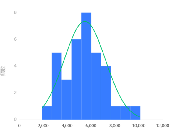
Figure 1 The histogram

The histogram above shows the normality test of the six categories, presenting a roughly bell-shaped curve (high in the middle, low at both ends), indicating that although the data is not perfectly normal, it is generally acceptable as a normal distribution. Therefore, we proceed with the Spearman correlation coefficient analysis.

Spearman correlation coefficient is applied to represent the relationship between category sales volumes, and the output result is presented as a correlation coefficient heatmap as follows:

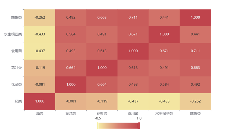
Figure 2 Heatmap

The heatmap above displays the values of the correlation coefficients, mainly represented by color depth. From -0.5 to 1.0, the color transitions from light to dark. A correlation coefficient > 0 indicates a positive correlation. The coefficients between cauliflower and leafy vegetables, aquatic root vegetables, leafy vegetables and edible fungi, edible fungi and aquatic root vegetables, chili peppers are all greater than 0.58, indicating a strong correlation between them. Cauliflower and edible fungi, chili peppers, leafy vegetables and aquatic root vegetables, aquatic root vegetables and chili peppers have correlation coefficients ranging from 0.4 to 0.5, indicating a moderate correlation between them. Except for itself, the correlation coefficients between tomatoes and the other five categories are all negative, indicating a negative correlation between tomatoes and the sales volumes of the other five categories.

4.1.2. Cluster Analysis model establishment

Due to the large monthly sales volume of individual items, here we apply K-means clustering analysis to classify the sales volume of individual items and compare their relationships. Cluster analysis is used to analyze the differences in clustering categories based on fields, then summarize the frequencies of each clustering category, and determine which category each sample data belongs to according to the clustering labels of the dataset. We aim to classify the 251 types of individual items based on the differences in sales volume, planning to divide them into three categories: moderate, high, and low total sales volume.

Cluster Scatter Plot

Based on the scatter plot of the two variables and analysis, it is evident that although there is some overlap between the three categories, the majority of category divisions have significant distinctions. From the cluster scatter plot, it is observed that the data of Category 1 is relatively dispersed, indicating a moderate relationship among the items in this category, with weak correlation. Category 2 data is more concentrated, indicating a strong correlation among the items in this category. The yellow dots represent the sales volume data of Category 3 items, which are highly dispersed. Due to the small number of low-sales items and their uneven distribution, items with moderate sales volume are the most numerous, indicating a stronger correlation among their sales volumes compared to the other two categories.

Field Differences Test

According to the results of quantitative field difference analysis (including mean ± standard deviation results, F-test results, significance P-values), the analysis of variance results show: for the variable “sales volume,” the significance P-value is 0.000***, indicating significance at the level, rejecting the null hypothesis, and demonstrating significant differences in sales volume between the categories defined by the cluster analysis. For the variable “individual items,” the significance P-value is 0.003***, indicating significance at the level, rejecting the null hypothesis, and demonstrating significant differences in individual items between the categories defined by the cluster analysis. Through the examination of the clustering model, it can be concluded that cluster analysis is feasible for this problem.

4.2 Model establishment and solution

4.2.1. Establishment of linear regression (least squares method)

In this study, each vegetable category is analyzed individually to examine the relationship between the total sales volume and cost-plus pricing. Let the independent variable be sales volume (X) and the dependent variable be unit price (Y). Since linear regression is used to study the linear relationship between the independent and dependent variables, data is imported into SPSSpro software to illustrate the relationship between sales volume and cost-plus pricing. By analyzing the F-value, it is determined whether the null hypothesis of a total regression coefficient being 0 can be significantly rejected (P < 0.05). If significant, it indicates a linear relationship. The strength of this relationship is further analyzed using the R² value to assess the model’s fit. The significance of X is analyzed; if significant (P < 0.05), it is used to explore the relationship between X and Y. The impact of X on Y is compared and analyzed with the regression coefficient (B) values.

1) Cauliflower Category

The analysis of the F-test results shows a significant p-value of 0.000***, indicating significance at the level. The null hypothesis of a regression coefficient of 0 is rejected, thus the model basically meets the requirements. Regarding the performance of variable collinearity, all Variance Inflation Factors (VIF) are less than 10, indicating no multicollinearity issues, and the model is well-constructed. The model formula is as follows:

y = 10.685 - 0.031*x, indicating a negative correlation between sales volume and cost-plus pricing for cauliflower.

2) Leafy Vegetables Category

The analysis of the F-test results reveals a significant p-value of 0.000***, indicating significance at the level. The null hypothesis of a regression coefficient of 0 is rejected, thus the model basically meets the requirements. Regarding the performance of variable collinearity, all Variance Inflation Factors (VIF) are less than 10, indicating no multicollinearity issues, and the model is well-constructed. The model formula is as follows:

y = 6.958 - 0.004*x, indicating a negative correlation between sales volume and cost-plus pricing for leafy vegetables.

3) Chili Peppers Category

The analysis of the F-test results shows a significant p-value of 0.000***, indicating significance at the level. The null hypothesis of a regression coefficient of 0 is rejected, thus the model basically meets the requirements. Regarding the performance of variable collinearity, all Variance Inflation Factors (VIF) are less than 10, indicating no multicollinearity issues, and the model is well-constructed. The model formula is as follows:

y = 11.049 - 0.009*x, indicating a negative correlation between sales volume and cost-plus pricing for chili peppers.

4) Tomatoes Category

The analysis of the F-test results shows a non-significant p-value of 0.876, indicating no significance at the level, and the null hypothesis of a regression coefficient of 0 cannot be rejected, rendering the model ineffective. Regarding the performance of variable collinearity, all Variance Inflation Factors (VIF) are less than 10, indicating no multicollinearity issues, and the model is well-constructed. The model formula is as follows:

y = 8.592 + 0.001*x, indicating a positive correlation between sales volume and cost-plus pricing for tomatoes.

5) Edible Fungi Category

The analysis of the F-test results shows a significant p-value of 0.000***, indicating significance at the level. The null hypothesis of a regression coefficient of 0 is rejected, thus the model basically meets the requirements. Regarding the performance of variable collinearity, all Variance Inflation Factors (VIF) are less than 10, indicating no multicollinearity issues, and the model is well-constructed. The model formula is as follows:

y = 13.492 - 0.019*x, indicating a negative correlation between sales volume and cost-plus pricing for the edible fungi category.

6) Aquatic Root Vegetables Category

The analysis of the F-test results shows a significant p-value of 0.000***, indicating significance at the level. The null hypothesis of a regression coefficient of 0 is rejected, thus the model basically meets the requirements. Regarding the performance of variable collinearity, all Variance Inflation Factors (VIF) are less than 10, indicating no multicollinearity issues, and the model is well-constructed. The model formula is as follows:

y = 11.743 - 0.037*x, indicating a negative correlation between sales volume and cost-plus pricing for the aquatic root vegetables category.

Conclusion:

Analyzing each category individually, it is observed that the monthly sales volume of tomatoes exhibits a linear negative correlation with cost-plus pricing, indicating that as the sales volume of tomatoes increases, their cost-plus pricing also increases. Similarly, for other categories, the sales volume exhibits a linear negative correlation with cost-plus pricing, suggesting that as the sales volume of other categories increases, their cost-plus pricing decreases.

4.2.2. Time series forecasting of daily replenishment volume

Replenishment planning is conducted on a category basis, based on the correlation data between the sales details of various products and wholesale prices. The total monthly sales volume of each vegetable category is integrated, and recent loss rate data for each product are considered. Using the formula:

Replenishment Volume = Sales Volume / (1 - Loss Rate),

the historical daily replenishment volume for each category can be determined. Time series analysis (ARIMA) is used to predict future data based on historical data. The ARIMA model automatically employs the Augmented Dickey-Fuller (ADF) test, which is used for stability testing and employs differential analysis to stabilize the data. Because the ARIMA model requires the series to be stationary, the ADF test results are examined to determine if the null hypothesis of non-stationarity can be significantly rejected (P < 0.05) based on the analysis of the t-value. Through time series analysis, the daily replenishment total for each vegetable category for the upcoming week can be forecasted.

1) Cauliflower Category

The model’s goodness of fit R² is 0.471, indicating a moderate model performance. Analysis reveals the predicted daily replenishment total for cauliflower over the next seven days as follows:

25.261272694369353, 22.575333045970677, 21.303306517191864, 20.691239467229057, 20.387215752910656, 20.22697464901126, 20.133845657813985 (kg)

2) Leafy Vegetables Category

Analysis indicates the predicted daily replenishment total for leafy vegetables over the next seven days as follows:

141.31187725523137, 130.59042843729668, 133.2398164322252, 135.81875569613894, 139.97363827943596, 141.60692317559668, 140.7793836995936 (kg)

3) Chili Peppers Category

Analysis shows the predicted daily replenishment total for chili peppers over the next seven days as follows:

87.10028082456598, 84.46916854686646, 82.1510016170741, 81.12231731690525, 84.83303545085879, 86.63559411164047, 86.72330458841634 (kg)

4) Tomatoes Category

The model’s goodness of fit R² is 0.548, indicating relatively good model performance. The predicted replenishment amounts for the next 7 days are:

24.121445688863027, 22.182147957211885, 18.830101150056723, 18.476353394562782, 17.794911737499973, 19.65169278501166, 20.695945680178415 (kg)

5) Edible Fungi Category

The model’s goodness of fit R² is 0.491, indicating moderate model performance. Predicted replenishment amounts for the next 7 days are:

49.056221598485806, 52.293470405796036, 53.55396392312175, 54.04509494998344, 54.236786463652955, 54.31193470523406, 54.34172375515646(kg)

6) Aquatic Root Vegetables Category

The model’s goodness of fit R² is 0.491, indicating moderate model performance. Predicted replenishment amounts for the next 7 periods are:

23.874274238541215, 24.86540755607719, 25.250955448355718, 25.62630972027943, 25.99173988413984, 26.347508326509363, 26.693870496640415 (kg)

4.2.3. XG-Boost Regression Model for Pricing Strategy

To establish pricing strategies for various vegetable categories based on the analysis of their sales volume and cost-plus pricing, aiming to maximize the revenue of supermarkets. XG Boost regression is a machine learning algorithm based on gradient boosting trees, primarily used for regression and classification problems. In solving optimization problems, the role of the XG Boost regression model is to predict the value of a continuous target variable. The XG Boost regression model can predict the value of the target variable based on input feature variables and provide functionalities such as feature importance assessment, outlier detection, and model interpretation.

The objective of the XG Boost regression model is to minimize the loss function, which is typically in the form of mean squared error (MSE) or log loss. Its mathematical formula can be expressed as follows:

\( Objective: min f(θ) = Ω(θ) + Σ(λ * α_{i} + γ * b_{i}) + Σ(L(y, F(x))) \)

Here, \( f(θ) \) represents the objective function of the model, where \( θ \) denotes the model parameters. \( Ω(θ) \) is the regularization term of the objective function, used to control the complexity of the model and prevent overfitting. It usually consists of two parts: the number of trees ( \( α_{i} \) ) and the depth of the trees ( \( b_{i} \) ). \( λ \) and \( γ \) are regularization parameters used to control the strength of these two parts. \( L(y, F(x)) \) is the loss function used to measure the difference between the model’s predicted value \( F(x) \) and the true value \( y \) . In regression problems, common loss functions include mean squared error and log loss. \( Σ \) denotes summation because XG-Boost constructs multiple decision trees, each corresponding to \( α \) and \( b \) values.

Based on time series analysis, the daily sales total from July 1st to July 7th is predicted. Then, considering the sales volume as the independent variable X and the unit price as the dependent variable Y.

1) Cauliflower Category

Based on the test data, the predicted unit prices for cauliflower sales over the next seven days are:

11.769662857055664, 8.100948333740234, 8.327664375305176, 12.691715240478516, 9.510427474975586, 9.753293991088867, 9.753293991088867 (Yuan)

2) Leafy Vegetables Category

Based on the test data, the predicted unit prices for leafy greens sales over the next seven days are:

6.34000301361084, 5.641404151916504, 7.475661277770996, 5.763496398925781, 6.34000301361084, 6.115345478057861, 6.441286087036133 (Yuan)

3) Chili Peppers Category

Based on the test data, the predicted unit prices for chili peppers sales over the next seven days are:

11.66492748260498, 8.743037223815918, 9.970579147338867, 19.634891510009766, 8.482512474060059, 8.482512474060059, 8.482512474060059 (Yuan)

4) Tomatoes Category

Based on the test data, the predicted unit prices for eggplant sales over the next seven days are:

8.379298210144043, 8.485044479370117, 9.539603233337402, 8.929167747497559, 12.131590843200684, 6.680470943450928, 7.9803314208984375 (Yuan)

5) Edible Fungi Category

Based on the test data, the predicted unit prices for mushroom sales over the next seven days are:

13.01437759399414, 13.516923904418945, 12.94736099243164, 13.550602912902832, 13.331441879272461, 13.331441879272461, 13.331441879272461 (Yuan)

6) Aquatic Root Vegetables Category

Based on the test data, the predicted unit prices for aquatic roots and stems sales over the next seven days are:

12.31882381439209, 11.983057975769043, 10.640172958374023, 7.9127984046936035, 11.261810302734375, 10.140564918518066, 10.21018123626709 (Yuan)

4.3. Other relevant data and suggestions

In order to better formulate replenishment and pricing decisions for vegetable products, supermarkets also need to collect the following relevant data:

1) Supply Chain Information for Vegetables: Supermarkets need to understand the supply chain information for vegetable products, including suppliers for each category, origin, transportation time, etc. This helps supermarkets assess the reliability of suppliers and product quality, choose stable supply channels, and adjust procurement plans promptly.

2) Inventory Data: Supermarkets need to collect inventory data for vegetable products, including inventory levels, inventory turnover rates, inventory costs, etc., to grasp inventory situations and optimize inventory management.

3) Consumer Data: Supermarkets need to collect information on consumer purchasing behavior, preferences, demands, etc., to understand consumer needs and formulate product strategies that better align with market demands.

4) Market Competition and Price Data: Supermarkets need to understand the market competition and price fluctuations, including competitors’ sales strategies and pricing methods. This helps supermarkets adjust their replenishment and pricing strategies, maintain competitiveness, and achieve reasonable profits.

5) Weather Data: Supermarkets need to collect weather data, including temperature, precipitation, etc., to analyze the impact of weather on vegetable sales and formulate corresponding sales strategies.

Regional Data: Supermarkets need to collect sales data and consumer demand information for different regions to formulate regional product and sales strategies.

6) Vegetable Quality and Shelf Life Information: Supermarkets need to collect relevant data on vegetable quality and shelf life, including ideal procurement cycles, shelf life, storage conditions, etc. This can help supermarkets better control the quality and shelf life of products and reduce loss rates.

7) Supply Sources and Procurement Timing Data: Supermarkets need to understand the supply sources and procurement timing for each vegetable category, which helps in making replenishment decisions. If a vegetable category from a particular supply source is often supplied at specific times and has high sales volume, supermarkets can increase the replenishment quantity accordingly to meet demand.

Quality Indicators for Vegetables: Supermarkets need to pay attention to indicators such as freshness, appearance quality, taste, and nutritional value of vegetables. These indicators can be obtained through testing and evaluation of vegetables, helping supermarkets determine whether products meet sales requirements.

In summary, the above data is very helpful for supermarkets to address replenishment and pricing decision-making issues.

5. Model evaluation

5.1. Advantages of the models

The Spearman correlation coefficient is a statistical method used to measure the non-linear relationship between two variables. It is widely applicable, as it can not only analyze the relationship between two continuous variables but also between two ordered or categorical variables. Moreover, the Spearman correlation coefficient does not rely on assumptions about the data distribution, thus allowing analysis of non-normally distributed or data with outliers. It has minimal sensitivity to outliers and is more robust compared to the Pearson correlation coefficient.

Cluster analysis does not require pre-labeled training data and can automatically discover patterns and structures within the data, making it suitable for exploratory data analysis and uncovering hidden information. Cluster analysis is based on the inherent features of the data itself and does not depend on prior knowledge or assumptions, enabling the discovery of underlying structures and relationships within the data.

Linear regression is a simple model that is easy to understand and interpret. It is based on linear relationships and can describe the relationship between variables through slope and intercept. The coefficients of the linear regression model can be used to explain the relationship between variables, determine the extent of the variables’ impact on the outcome based on the sign and magnitude of the coefficients, and predict the value of the dependent variable. When input variables change, the model can predict the change in the outcome.

5.2. Disadvantages of the models

The Spearman correlation coefficient can only measure the monotonic relationship between variables and cannot accurately reflect the strength and direction of linear relationships. When the sample size is small, the estimation of the Spearman correlation coefficient may not be accurate enough, leading to potential misjudgments. The Spearman correlation coefficient requires complete pairing of data for two variables, and missing values necessitate data processing or deletion.

Cluster analysis requires the selection of appropriate initial parameters, such as the number of clusters and distance measures, which may lead to different results, requiring multiple attempts and evaluations. Cluster analysis is sensitive to noise and outliers, which may affect the accuracy and stability of the clustering results.

The linear regression model assumes the existence of a linear relationship between variables, but the actual relationship in the data may be non-linear. If the data does not meet the linear assumption, the predictive ability of the linear regression model may be limited. The linear regression model is sensitive to outliers, and the presence of an outlier may significantly affect the model’s fit.

6. Conclusion

This paper employs models such as Spearman correlation coefficient, cluster analysis, linear regression, and time series analysis to study the problem. Firstly, the distribution patterns and relationships among sales volumes of various vegetable categories and individual products are analyzed through the Spearman correlation coefficient and cluster analysis models. Based on this foundation, the linear regression model is used to present the relationship between sales volume and pricing. Additionally, time series analysis is employed to forecast daily replenishment quantities, followed by XG-Boost regression for pricing prediction. This approach provides optimized solutions for replenishment and pricing decisions for supermarkets. Finally, this paper also discusses other relevant factors that may affect vegetable replenishment and pricing decisions, helping decision-makers better understand market and consumer demands, as well as supply chain and production situations, thereby formulating more rational replenishment and pricing strategies.

References

[1]. Scientific Platform Serving for Statistics Professional. (2021). SPSSPRO (Version 1.0.11) [Online Application Software]. Retrieved from https://www.spsspro.com.
[2]. Xu, W. C. (2012). A Review of Correlation Coefficients Research. Journal of Guangdong University of Technology, 29(3), 12-17.
[3]. Scientific Platform Serving for Statistics Professional. (2021). SPSSPRO (Version 1.0.11) [Online Application Software]. Retrieved from https://www.spsspro.com.
[4]. Saroj, K., & Kavita. (2016). Review: Study on Simple K Mean and Modified K Mean Clustering Technique. International Journal of Computer Science Engineering and Technology, 6(7), 279-281.
[5]. Scientific Platform Serving for Statistics Professional. (2021). SPSSPRO (Version 1.0.11) [Online Application Software]. Retrieved from https://www.spsspro.com.
[6]. Wang, Y. (2005). Application of Time Series Analysis. Beijing: China Renmin University Press.
[7]. Scientific Platform Serving for Statistics Professional. (2021). SPSSPRO (Version 1.0.11) [Online Application Software]. Retrieved from https://www.spsspro.com.
[8]. Chen, T., & Guestrin, C. (2016). XGBoost: A Scalable Tree Boosting System. ACM.
[9]. Scientific Platform Serving for Statistics Professional. (2021). SPSSPRO (Version 1.0.11) [Online Application Software]. Retrieved from https://www.spsspro.com.
[10]. Draper, N. R., & Smith, H. (1998). Applied Regression Analysis. Wiley Series in Probability and Statistics.
Cite this article
Long,C. (2024). Optimization research on automatic pricing and replenishment decision method for vegetable commodities. Advances in Engineering Innovation,7,48-54.
Data availability
The datasets used and/or analyzed during the current study will be available from the authors upon reasonable request.
Disclaimer/Publisher's Note
The statements, opinions and data contained in all publications are solely those of the individual author(s) and contributor(s) and not of EWA Publishing and/or the editor(s). EWA Publishing and/or the editor(s) disclaim responsibility for any injury to people or property resulting from any ideas, methods, instructions or products referred to in the content.
About volume
Journal:Advances in Engineering Innovation
© 2024 by the author(s). Licensee EWA Publishing, Oxford, UK. This article is an open access article distributed under the terms and
conditions of the Creative Commons Attribution (CC BY) license. Authors who
publish this series agree to the following terms:
1. Authors retain copyright and grant the series right of first publication with the work simultaneously licensed under a Creative Commons
Attribution License that allows others to share the work with an acknowledgment of the work's authorship and initial publication in this
series.
2. Authors are able to enter into separate, additional contractual arrangements for the non-exclusive distribution of the series's published
version of the work (e.g., post it to an institutional repository or publish it in a book), with an acknowledgment of its initial
publication in this series.
3. Authors are permitted and encouraged to post their work online (e.g., in institutional repositories or on their website) prior to and
during the submission process, as it can lead to productive exchanges, as well as earlier and greater citation of published work (See
Open access policy for details).