1 Introduction

1.1 Research Background

With the increasing emphasis on infrastructure construction and the development of emerging industries, power cables are expected to be widely used in the future, providing new opportunities for the electrical equipment and cable industry. Unlike traditional overhead lines, power cables are generally buried underground but can still develop defects over long-term operation due to various reasons, including mechanical damage, aging, environmental impact, and electrical stress [1]. Common cable defects include insulation aging, outer sheath damage, partial discharge, and conductor corrosion. These defects can reduce cable efficiency and may even cause power failures and accidents.

Timely monitoring of cable defects can prevent the occurrence and spread of faults, ensuring the safe and stable operation of the power system. Power failures typically result in significant economic losses; effective monitoring and early diagnosis can reduce maintenance costs and power outage losses. Regular monitoring and maintenance can also significantly extend the cable's service life and improve asset utilization. Thus, monitoring cable faults and identifying their types is crucial for the stable operation of the power system [2].

Early cable monitoring mainly relied on manual inspections and periodic tests such as infrared detection and partial discharge testing. With technological advancements, many advanced monitoring techniques have emerged, such as online monitoring systems, smart sensors, and big data analysis. These technologies enable real-time monitoring of cable operating conditions, fault prediction, and diagnosis.

1.2 Current Research Status

Research on power cable fault monitoring technology has long been a key topic in the power system field. In recent years, with technological advancements, the research content and applications have been continuously deepened and expanded. Modern cable fault monitoring systems are gradually developing towards intelligence, integrating various sensing technologies and intelligent algorithms.

Partial Discharge Monitoring: By detecting partial discharge signals, it is possible to determine whether there are defects inside the cable. Partial discharge can be caused by insulation material defects, such as corona discharge, surface discharge, floating discharge, and internal discharge. Common methods include ultrasonic detection, ground potential detection (GPR), and electromagnetic wave detection [3]. Partial discharge can not only cause insulation damage but also lead to more severe faults. Therefore, timely detection and localization of partial discharge are essential for ensuring normal cable operation [4].

Optical Fiber Sensing Technology: By arranging optical fiber sensors inside the cable, it is possible to monitor parameters such as temperature and strain in real time and determine defects. Distributed optical fiber sensors (DTS, DSS) are widely used in this field. For example, studies on optical fiber grating (FBG) and Sagnac interference show that these technologies can effectively detect partial discharge in cables [4].

Cable Fault Localization Algorithms: These algorithms use the principle of electromagnetic wave reflection and employ techniques such as Time-Domain Reflectometry (TDR) and Frequency-Domain Reflectometry (FDR) to locate cable faults. These methods can accurately locate fault positions without damaging the cable, significantly improving the efficiency and accuracy of cable fault handling. For example, a real-time monitoring and localization system based on all-fiber sensing technology can monitor the health status of cables and locate leakage positions in real-time [5].

As cable monitoring technology progresses, temperature field monitoring has gradually become an important research direction. In urban power grids, there may be dozens of cables in the same cross-section, with strong electromagnetic coupling and thermal effects between cables. Additionally, cables are laid in various ways and exposed to complex external environments, where heat transfer may involve conduction, radiation, and convection simultaneously.

The conductor temperature is a crucial indicator of cable life, and cable temperature is also an important basis for determining current-carrying capacity. By establishing a temperature field model of power cables based on real-time sensing data, it is possible to analyze cable temperature states in real-time and predict cable operating conditions and short-term current-carrying capacity, significantly enhancing the digital management level of cables [6]. Temperature field monitoring technology studies the temperature distribution during cable operation. Monitoring the temperature field can improve cable safety and reliability and provide crucial technical support for the stability and efficient operation of the power grid. Thus, research on temperature field monitoring technology has significant practical significance and application prospects.

1.3 Research Significance

With the rapid development of the power system and the continuous transformation of the energy structure, modern power network structures are becoming increasingly complex and expanding in scale. Transmission lines are becoming more critical to the entire power system, and as a vital component of transmission lines, the reliability and safety of power cables directly affect the stability of the power system. However, as usage time increases, power cables may develop defects due to various reasons, which can reduce insulation performance and potentially lead to severe power accidents. Therefore, the study of temperature field monitoring technology has important practical significance and application prospects.

1. Preventing Overheating Faults: High temperatures can cause insulation material to age or fail. Monitoring temperatures can help detect and address overheating issues in time to prevent faults.

2. Real-time Monitoring: Temperature monitoring systems enable 24-hour real-time monitoring of cables, allowing for early detection of abnormal temperature rises and providing early warnings.

3. Extending Cable Life: Controlling operating temperatures can reduce the damage to insulation materials, thus extending cable service life.

4. Improving System Reliability: Timely detection and handling of abnormal cable temperatures can reduce outages and maintenance costs, enhancing the overall reliability of the power system.

5. Fault Localization: Abnormal temperatures are often precursors to cable faults. Temperature monitoring can quickly locate fault areas, reducing troubleshooting time.

6. Optimizing Load Management: Monitoring cable temperatures can help optimize power load distribution, avoiding overheating due to unbalanced loads.

Therefore, temperature monitoring, as a critical means of detecting cable faults, can significantly enhance the safety and stability of cable systems and is a key technology in power system maintenance and management.

During the production of cable terminals or intermediate joints, the original structural layers must be stripped, which may scratch the insulation layer and create air gaps, resulting in uneven electric field distribution on the insulation surface, discharge, abnormal temperature rise, and material aging. These phenomena can affect the performance of the cable insulation layer. According to statistics, about 70% of cable accidents occur at cable accessories.

Therefore, analyzing the electric field and temperature distribution at cable joints is crucial for studying and monitoring cable faults. Based on this, this paper focuses on monitoring and analyzing the temperature field of power cables under different defect conditions.

2 Comsol Simulation Analysis of Cable Temperature Field

2.1 Physical Model of the Cable

Taking the YJLW 64/110kV single-core cable as an example, a simulation analysis is conducted. Due to the high thermal conductivity, small geometric thickness, and low thermal resistance of the cable's armor and shielding layers, their impact on the temperature field distribution is minimal. Therefore, they are neglected in the physical modeling for simplification. The basic structure of the cable includes the conductor, insulation layer, metal sheath layer, and outer sheath layer [7]. The origin of the simulation model coordinates is set at the center of the cable. The established simplified two-dimensional cable model is shown in Figure 2.1.

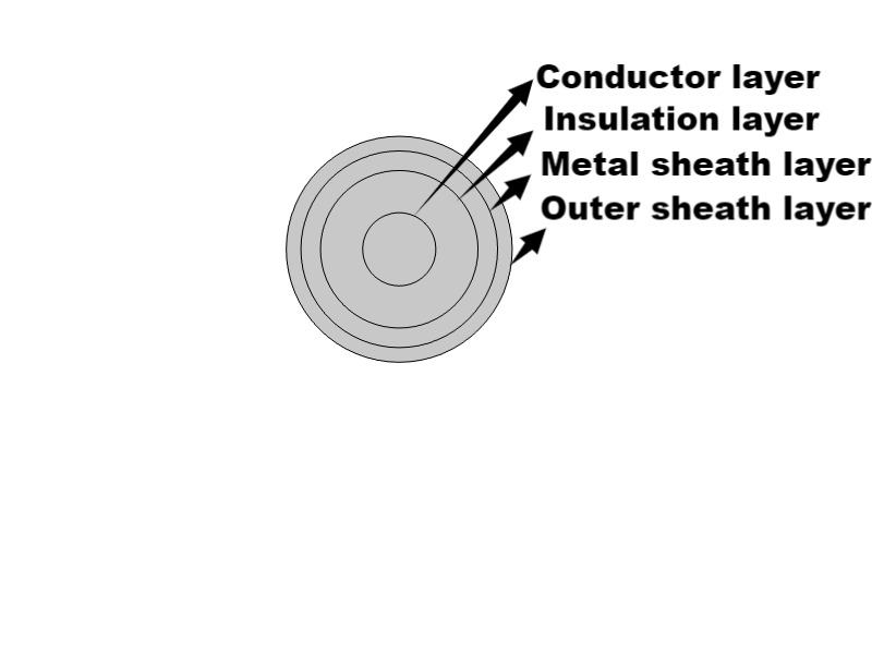
Figure 1. Cable physical model diagram

In the physical model, the parameter settings for each part are as follows:

The center of the cable is the conductor, typically made of copper or aluminum, responsible for transmitting electrical energy. The size and material of the conductor depend on the cable's rated current and voltage. In this model, the conductor material is set to copper, with a conductor radius of 8.75mm. Other electrical and thermal parameters are shown in Figure 2.2.

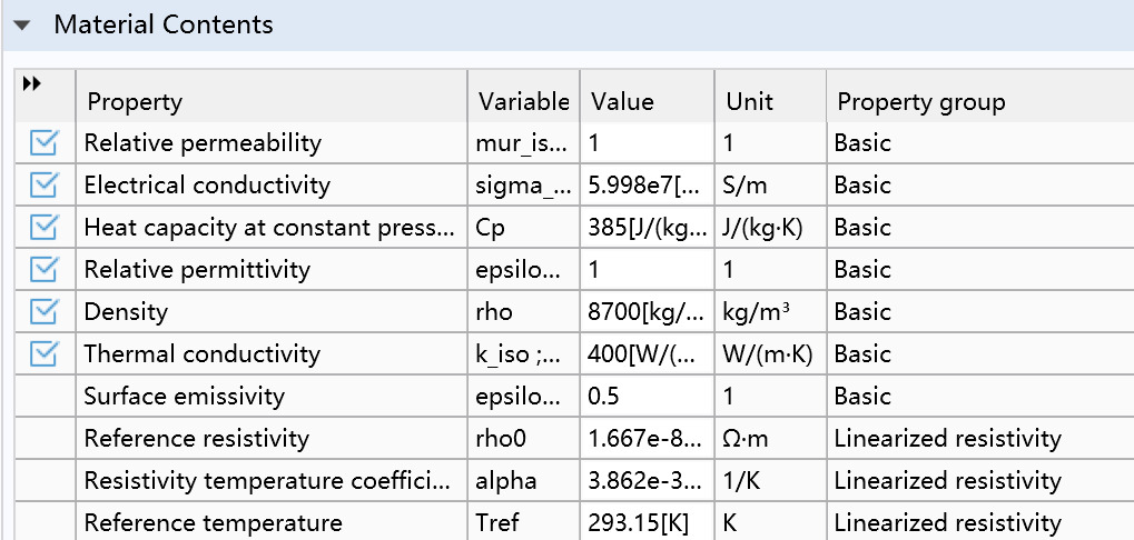
Figure 2. Copper conductor-related parameters

Insulation Layer: Around the conductor is one or more layers of insulation material to prevent current leakage and protect the cable from external environmental influences. Insulation materials are usually cross-linked polyethylene (XLPE) or polyvinyl chloride (PVC), known for their good electrical insulation properties and chemical stability. The insulation layer radius is set to 7.95mm, with other electrical and thermal parameters shown in Figure 2.3.

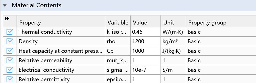
Figure 3. Relevant parameters of the insulation layer

Metal Sheath Layer: Outside the insulation layer is the metal sheath layer, typically made of lead or aluminum. The metal sheath layer provides additional protection, preventing moisture and other harmful substances from entering the cable and reducing electromagnetic interference. The metal sheath layer radius is set to 4.00mm, with other electrical and thermal parameters shown in Figure 2.4.

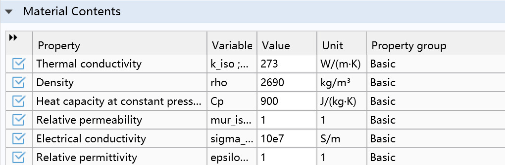
Figure 4. Relevant parameters of the metal sheath layer

Outer Sheath Layer: The outermost layer is the outer sheath layer, usually made of polyethylene (PE) or polyvinyl chloride (PVC), providing mechanical protection against physical damage and resistance to UV rays and chemical corrosion. The outer sheath layer radius is set to 2.80mm, with parameters set the same as the insulation layer.

2.2 Physical Field Parameters and Simulation Settings

2.2.1 Heat Source

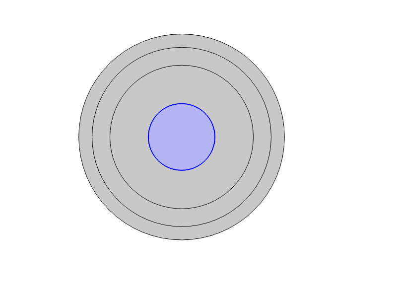
Figure 5. Heat source model

In the study of the temperature field of power cables, the heat source mainly comes from the Joule heat generated by the cable conductor resistance under current excitation.

The conductor layer cable core is shown in Figure 2.5. In cable design, specific electrical and mechanical standards dictate the maximum current the cable can safely carry. The current-carrying capacity of the cable must meet the needs of its application. In this study, the coil excitation is chosen in the form of current, with the coil current set \( I_{coil} \) to 2000A according to the GB 50217 (2018) electrical engineering cable design standards.

In practical applications, 2000A is a relatively high current value, usually used for special applications or specific conditions. In most standard applications, the rated current of the cable may be significantly lower. When designing and selecting cables, practical current needs, safety standards, and economic factors should be considered. The effect of changing the coil current \( I_{coil} \) on the heat generated by the cable can be studied directly. The basic Joule heat formula is as follows:

\( Q=I^{2}Rt \) (2.1)

where Q represents the heat generated over time, and R represents the resistance of the conductor.

It should be noted that the actual current-carrying capacity of the cable also needs to consider multiple factors, including laying conditions, surrounding environment, laying depth, thermal resistance of the soil or water, and safety margins. These factors can affect the cable's thermal performance and ultimate current-carrying capacity. For more precise calculations of the cable's thermal behavior, more complex thermal models and equations are required.

The conduction model is set to the form of conductivity, expressed in the differential form of Ohm's law:

\( J_{c}=σE \) (2.2)

where \( J_{c} \) represents the current density, indicating the current passing through a unit area. The conductivity \( σ \) is set according to the copper conductor-related parameters. The cable's temperature field distribution is primarily established through thermal conduction.

Thermal conduction formula:

\( -n∙q=d_{z}q_{0}=∆Q \) (2.3)

2.2.2 Temperature Field Boundary Conditions

During operation, the cable generates heat that needs to be dissipated effectively to maintain safe operation and extend its lifespan. In the temperature field simulation model, the heat exchange between the cable surface and the external environment is typically represented as convective heat transfer. The temperature field boundary condition is given by the convective heat formula:

\( q=h(T_{ext}-T) \) (2.4)

Herein, n is the unit normal vector, indicating the positive direction of heat transfer. q is the heat flux density, representing the heat flow per unit area. \( ∆Q \) is the amount of heat passing through a certain area per unit time. h is the heat transfer coefficient, and \( T_{ext} \) denotes the external temperature.

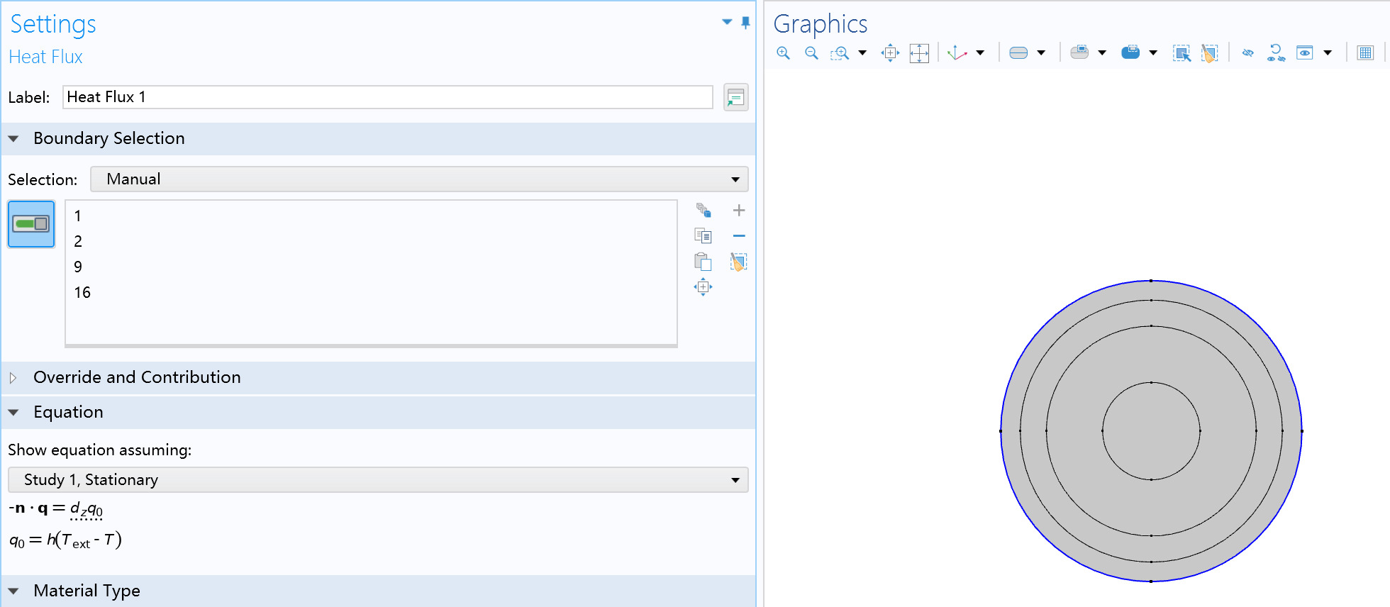
Figure 6. Set up the convective heat flux

In COMSOL, the flux type is set to convective heat flux, with the heat transfer coefficient ℎempirically set at \( 15W/(m^{2}∙k) \) , and the external temperature set to 303.15K, assuming an external environment temperature of 30°C.

2.2.3 Meshing

In COMSOL, the mesh is used to discretize the continuous physical domain (such as space or time) into a finite number of small elements or nodes. This discretization forms the basis for numerically solving continuous problems. The shape and size of the mesh can adapt to different physical properties and boundary conditions, such as using finer mesh near geometric features to capture details. In this study, the mesh visualizes the cable's temperature field distribution, helping users understand the simulation results intuitively. The mesh scale determines the calculation complexity and required computational resources. Reasonable meshing can balance calculation accuracy and efficiency, and is crucial for achieving accurate and efficient numerical simulations. The finite element section results of the cable model are shown in Figure 2.7.

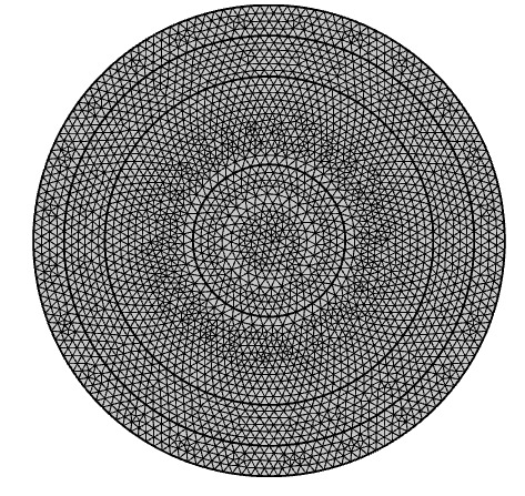
Figure 7. Cable finite element section results

The statistics of each unit are shown in Figure 2.8.

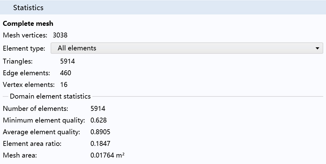
Figure 8. Cell information statistics Fig

It can be seen that in the temperature field simulation calculation under normal cable operating conditions, the triangular finite element model has a large scale, containing both the number of units and nodes in the same order of magnitude: \( 10^{4} \) .

2.2.4 Solver Settings

In COMSOL, the steady-state solver is used to solve physical problems that do not change over time. The steady-state parameter settings are shown in Figure 2.9.

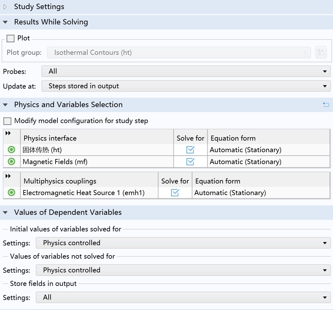
Figure 9. Steady-state parameter setting

In COMSOL solver configuration, the nonlinear method is chosen as automatic (Newton), with the initial damping factor set to 0.01, the minimum damping factor set to 1E-6, the update step size limit set to 10, the step size growth limit set to 1, the automatic use of recovery damping factor set to 0.75, the termination technique set to tolerance, the maximum number of iterations set to 50, and the tolerance factor set to 1. The solver chosen is GMRES. The final steady-state temperature distribution solved by the steady-state solver is shown in Figure 2.10.

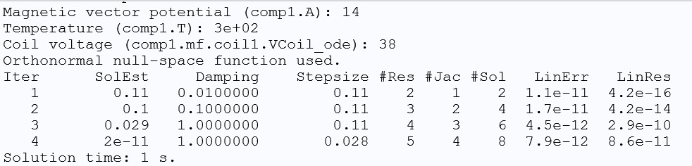
Figure 10. Steady-state solver result

2.2.5 Post-Processing

After completing the temperature field simulation, the temperature field distribution can be visually displayed through two-dimensional contour maps and one-dimensional line diagrams. For example, in the simulation results of the temperature field of a normal cable, the two-dimensional contour map is shown in Figure 2.11.

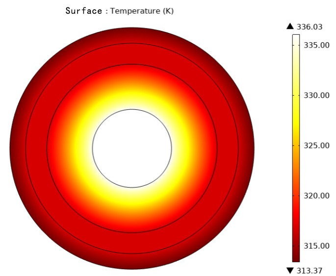
Figure 11. Two-dimensional contour of the temperature distribution on the cable surface

The one-dimensional line diagram is shown in Figure 2.12.

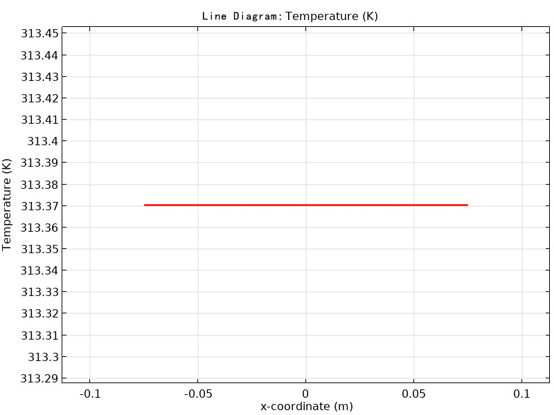
Figure 12. Cable surface temperature distribution line diagram

2.3 Simulation Analysis of the Temperature Field under Normal Conditions

According to formula 2.1, when only the coil current \( I_{coil} \) changes and other parameters remain unchanged, the surface temperature of the cable will change. The variation pattern is shown in Figure 2.13.

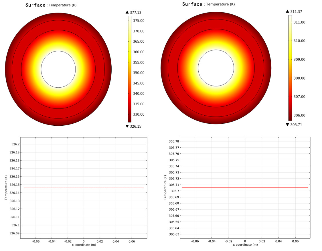
(a) \( I_{coil} \) =3000A (b) \( I_{coil} \) =1000A

Figure 13. Cable temperature field and cable surface temperature distribution

It is clear from the above figure that when the coil current \( I_{coil} \) is 3000A, the cable surface temperature is approximately 326.15K, while at 1000A, the surface temperature is approximately 305.71K. The simulation results reveal that the relationship between the coil current \( I_{coil} \) and the cable surface temperature is not linear. When the coil current \( I_{coil} \) increases, the temperature gradient across the cable section increases, yet the surface temperature of the cable remains relatively constant, with the temperature distribution of the conductor, insulation, and metal sheath layers remaining uniform. Conversely, when the coil current \( I_{coil} \) decreases, the temperature gradient also decreases, in accordance with the physical laws described by formula 2.1.

Using a one-dimensional line diagram, the trend of temperature changes on the cable surface can be clearly seen, while the two-dimensional contour map represents the temperature distribution across the entire cable section. However, in practical engineering problems, it is difficult to measure the internal temperature of the cable, so choosing the cable surface temperature as the fault diagnosis basis is more aligned with engineering practices.

According to formula 2.4, when only the heat transfer coefficient ℎ changes and other parameters remain unchanged (with the coil current \( I_{coil} \) set to 2000A), the surface temperature of the cable will change. The variation pattern is shown in Figure 2.14.

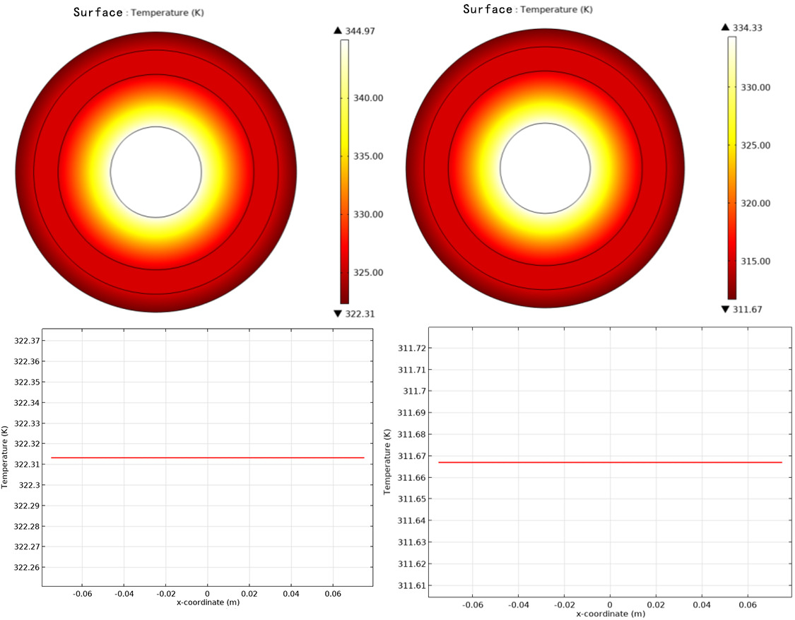
(a)heat transfer coefficient h=8 (b)heat transfer coefficient h=18

Figure 14. Cable temperature field and cable surface temperature distribution

It is clear from the above figure that when the heat transfer coefficient is 8, compared to ℎ being 15, the surface temperature of the cable rises, and the temperature gradient across the entire cable section increases. Conversely, when the heat transfer coefficient ℎ is 18, compared to ℎ being 15, the surface temperature of the cable decreases, and the temperature gradient across the entire cable section decreases. This is because the heat transfer coefficient ℎh describes the heat flow per unit area per unit temperature difference, representing the convective heat transfer capacity. If the heat transfer coefficient ℎ decreases, it means that the fluid's (e.g., air or water) ability to carry away heat under the same temperature difference condition decreases. Conversely, if ℎ increases, the fluid's ability to carry away heat increases. The simulation results conform to the physical laws described by formula 2.4.

2.4 Simulation Analysis of the Temperature Field under Internal Defects

2.4.1 Eccentric Defect

Under normal conditions (ideal conditions), the cable model presents concentric circles, where the center of each layer of the cable section is located at the same position. However, in practical engineering problems, due to manufacturing process differences, material inconsistencies during cable manufacturing, and uneven mechanical loads or thermal stress during long-term operation, the conductor material may become asymmetrical, leading to eccentricity. This is illustrated in Figure 2.15.

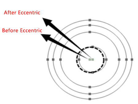
Figure 15. Comparison diagram before and after cable eccentric

Cable eccentricity, where the conductor is offset relative to the center of the cable sheath or insulation layer, may cause uneven surface temperature distribution. After cable eccentricity, the insulation thickness inside the cable varies, altering the heat conduction path from the conductor to the sheath, which may reduce the efficiency of heat transfer within the cable. Simultaneously, the cable's heat dissipation primarily occurs through the sheath or insulation layer. If the conductor is eccentric, the dissipation area in some regions may reduce, affecting the effective heat dissipation, and ultimately causing uneven surface temperature distribution, potentially impacting the cable's performance and safety. In the temperature field simulation of a cable with eccentric defects, the surface convection coefficient is set as \( h=15W/(m^{2}∙k) \) , the external temperature is set to 303.15K, and the cable current-carrying capacity is 2000A. The simulation results are shown in Figure 2.16.

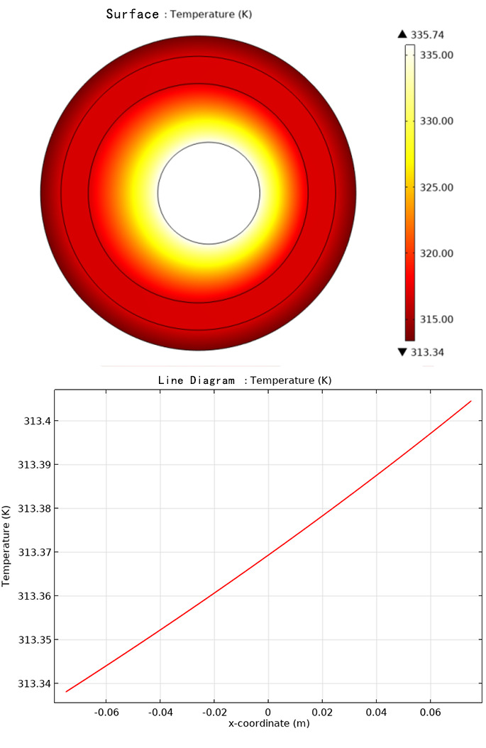
Figure 16. Surface temperature distribution after cable eccentric

From the simulation results of the temperature field, it can be seen that the surface temperature distribution of cables with eccentric defects is uneven [7]. The surface temperature of the cable near the new center, where the insulation thickness is thin, increases, reaching a maximum of 313.405K. Conversely, the surface temperature of the cable far from the new center, where the insulation thickness is thick, decreases, with a minimum of 313.335K. It is evident that the temperature distribution difference caused by eccentricity is very small, only 0.07K. When using temperature to detect the degree of cable eccentricity in practical engineering problems, it requires temperature detection equipment with high sensitivity. Considering factors such as cost-effectiveness in practical engineering problems, it is challenging to detect cable eccentricity defects through temperature measurement.

2.4.2 Water Tree Defects

Water treeing is a branch-like aging phenomenon that develops in the insulation material of cables, usually associated with moisture or chemical contaminants. Under normal conditions, the external conductor layer of the cable is insulating. However, during manufacturing, installation, or operation, the cable may be exposed to moist environments. Moisture penetrates into the cable through tiny defects in the sheath or insulation layer. Over time, as the cable operates, its physical and chemical properties deteriorate, gradually forming water trees and being affected by them. The water tree has a branch-like shape and is simulated in the model using elongated ellipses of random shapes and positions to represent the water tree and the surrounding aged insulation material [7]. This is illustrated in Figure 2.17.

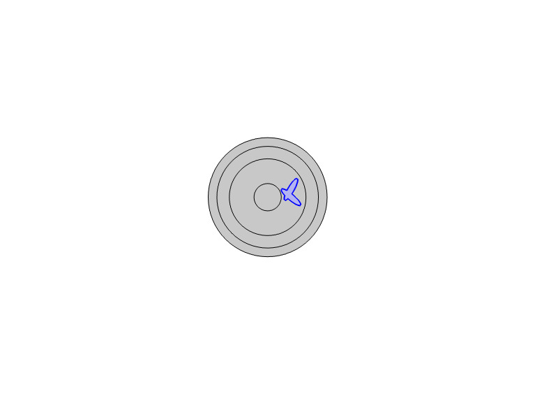
Figure 17. Cable-generated water branch defect model

The presence of water trees may disrupt the uniformity of the insulation material, reduce thermal conductivity efficiency, and cause heat to accumulate in certain areas. If water trees cause the cable surface to become uneven or form protrusions, this may alter airflow patterns and affect heat dissipation, resulting in uneven temperature distribution. Ultimately, this leads to a decline in cable performance. Additionally, the number and location of water trees will also affect the surface temperature distribution of the cable. In the temperature field simulation of cables with water tree defects, the surface convection coefficient is set as \( h=15W/(m^{2}∙k) \) , the external temperature is set to 303.15K, and the cable current is 2000A. The simulation results are shown in Figure 2.18.

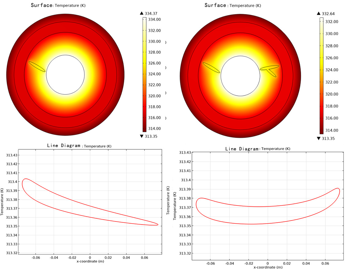
(a) Single Defect (b) Double Defects

Figure 18. Cable temperature field and cable surface temperature distribution

From the simulation results of the temperature field, it can be seen that when water tree defects are present inside the cable, the temperature field distribution becomes distorted. The one-dimensional line graph is no longer a straight line compared to the normal operating state [7]. Additionally, the surface temperature distribution of the cable shows significant differences from the normal operating state. In both single defect and double defect states, the surface temperature near the defects is higher, reaching approximately 313.4K. Therefore, in practical engineering problems, the characteristics of the cable surface temperature distribution under different water tree defects can be used to effectively identify the type of internal faults in the cable.

3 Conclusion

The surface temperature field distribution of power cables operating with local defects differs from that in normal operating conditions. This paper constructs a two-dimensional simulation model of the power cable cross-section to analyze the surface and internal temperature fields of power cables under normal and typical defect conditions (eccentric defects, internal water tree defects). The results indicate that temperature field variations are highly sensitive to internal defect characterization. The temperature field model can effectively locate and identify the types of internal defects in cables, demonstrating the potential of temperature field analysis in monitoring internal cable defects. As a non-invasive detection method, it does not require physical cutting or damage to the cable. Therefore, detecting internal defects in power cables based on temperature field analysis is an efficient and economical method that can significantly improve the operational efficiency and safety of cable systems.

References

[1]. Zhang, G., & Zhong, H. (2016). Analysis of the advantages and disadvantages of using cables or overhead lines in urban power lines. Mechanical & Electrical Engineering Technology, 45(11), 118-122.
[2]. Wang, H. (2022). Research on XLPE cable partial discharge pattern recognition based on SSDAE algorithm. Dalian University of Technology. https://doi.org/10.26991/d.cnki.gdllu.2022.002641
[3]. Jiang, Y. (2019). Research on cable partial discharge detection and localization system. Beijing Jiaotong University.
[4]. Li, R. (2020). Research on cable partial discharge detection method based on optical fiber sensing technology. North China Electric Power University (Beijing). https://doi.org/10.27140/d.cnki.ghbbu.2020.001178
[5]. Chen, Z., Song, Y., Peng, Y., et al. (2021). Real-time monitoring and localization system for cable leakage based on all-optical sensing technology. China Equipment Engineering(04), 175-177.
[6]. Huang, L., Liang, Y., Huang, H., et al. (2024). Rapid calculation method of power cable temperature field based on surrogate model and its application. Electric Power, 57(05), 178-187.
[7]. Jiang, Y., Fang, Y., Zhao, W., et al. (2022). Research on power cable defect detection method based on inverse temperature field problem. Advanced Technology of Electrical Engineering and Energy, 41(09), 81-88.
Cite this article
Li,Z. (2024). Analysis of internal defects in power cables based on temperature field simulation. Advances in Engineering Innovation,10,36-48.
Data availability
The datasets used and/or analyzed during the current study will be available from the authors upon reasonable request.
Disclaimer/Publisher's Note
The statements, opinions and data contained in all publications are solely those of the individual author(s) and contributor(s) and not of EWA Publishing and/or the editor(s). EWA Publishing and/or the editor(s) disclaim responsibility for any injury to people or property resulting from any ideas, methods, instructions or products referred to in the content.
About volume
Journal:Advances in Engineering Innovation
© 2024 by the author(s). Licensee EWA Publishing, Oxford, UK. This article is an open access article distributed under the terms and
conditions of the Creative Commons Attribution (CC BY) license. Authors who
publish this series agree to the following terms:
1. Authors retain copyright and grant the series right of first publication with the work simultaneously licensed under a Creative Commons
Attribution License that allows others to share the work with an acknowledgment of the work's authorship and initial publication in this
series.
2. Authors are able to enter into separate, additional contractual arrangements for the non-exclusive distribution of the series's published
version of the work (e.g., post it to an institutional repository or publish it in a book), with an acknowledgment of its initial
publication in this series.
3. Authors are permitted and encouraged to post their work online (e.g., in institutional repositories or on their website) prior to and
during the submission process, as it can lead to productive exchanges, as well as earlier and greater citation of published work (See
Open access policy for details).