1.Introduction

Machine learning is an interdisciplinary field that is unprecedentedly active in recent years. After decades of progress, the application scale of machine learning has been largely enhanced. As a discipline that studies computers’ simulation of human learning process and improvement of their performance, machine learning has become a useful assistant in industries, and an influencer of human life.

Machine learning can be applied to a wide range of industries. In biology field, Hazarika et al. proposed a visual analysis system that can help with the analysis of a yeast cell polarization simulation by immediately interacting with biologists. They trained a neural network-based surrogate model that can serve as the backend analysis framework, and used it to perform interactive parameter sensitivity analysis. The activation maximization framework was used to recommend optimal parameter configurations. The parameter configurations they discovered generated strong cell polarization results. They integrated their visual analysis workflow with that of the experts [1]. In order to make small utilities without technical knowledge understand how machine learning can forecast energy demand and supply, Grimaldo et al. designed a tool for short-term energy demand forecasting in prosumer scenarios that both generates forecasts and provides visual analytics, allowing utility analysts to know the process and criteria of those forecasts. They also presented a prototypical implementation of this approach [2]. Besides, machine learning has been suggested to assist data visualization. Wang et al. figured out seven main visualization processes that can be assisted by applying machine learning techniques. Then the seven processes were connected to existing visualization models to form a pipeline. Also, in order to reveal how ML is used to solve visualization problems, they map the seven visualization processes into different types of ML tasks [3].

Even during COVID-19, machine learning offered great help to human beings. Ndiaye et al. firstly analyzed public data in detail and visualized them. They focused on active cases, high-density areas, morality rate, growth factors, etc. Then they used different machine learning technics (linear regression, polynomial regression, support vector regression, prophet, and multilayer perception) to forecast the inflection point and confirmed cases of COVID-19 in two weeks and 40 days in Senegal [4].

Humans’ daily life can be optimized by machine learning in many aspects. Zheng et al. proposed a Deep Q-Learning based recommendation framework, to address three major problems of news recommendation: only model current reward; use click/no click labels but not user feedback; recommend similar news. They applied a DQN structure; taken user activeness into consideration; replaced classical exploration methods by a method called Dueling Bandit Gradient Descent. Their learning framework focuses on both present and future reward, has higher accuracy, and avoids recommending highly similar news [5]. Smart et al. developed a tool that uses a seed color to help designers automatically generate effective color ramps. They constructed a corpus of 222 high-quality designer-crafted color ramps, then normalized and clustered it. They constructed a model based on the results and seeded it. They evaluated their model by conducting an empirical study that compare the outputs of their model with those of designers, and found that their model is of accuracy and aesthetical value [6]. Wu et al. proposes MobileVisFixer to make visualizations more mobile-friendly. They classified mobile-friendly issues into five categories. MobileVisFixer addresses four of these issues on single Cartesian visualizations with linear or discrete scales. MobileVisFixer deconstructs charts into declarative description of visualizations, and then with the incorporation of reinforcement learning framework, forms mobile-friendly designs. The effectiveness, explainability, and generalizability of MobileVisFixer are demonstrated by quantitative evaluation on two real-world datasets [7].

In certain areas, models can be almost as good as humans. By adopting the deep learning (DL) framework, especially the explicit 3D modeling for facial alignment, and using a large dataset of faces for training, Taigman et al. developed a nine-layer deep neural network that contains locally connected layers instead of the commonly seen convolutional ones. In the Labeled Faces in the Wild benchmark (LFW), the accuracy of the network approached human level [8].

Algorithms are designed and improved, and as the available computing power increases, more complex models are trained. Marco Tulio Ribeiro et al. proposed LIME, a novel algorithm that can faithfully explain the predictions of any classifier or regressor. They further proposed SP-LIME, a method that can select multiple individual predictions and offer explanations to them. Users can judge those explanations and decide whether the model producing those predictions is trustworthy. In their experiments, they tested the practicality of the method and found users can pick and even improve classifiers successfully [9]. Gui et al. provides a review of generative adversarial network methods with a focus on algorithms, theory, and applications. GANs have many representative variants, and is hard to train. GANs use maximum likelihood estimation, and can suffer from model collapse and other theoretical issues, like memorization. GANs can be applied to fields like image processing, computer vision, sequential data, for they do not need explicit true data distribution or prior mathematical assumptions [10]. Krizhevsky et al. used a large dataset to train one of the largest convolutional neural networks (CNNs). They chose a highly optimized GPU and used effective ways to prevent overfitting. Their final network contains five convolutional and three fully connected layers, and when being applied to classify the images in the ImageNet ILSVRC-2010 and ILSVRC-2012 competitions, it achieved by far the lowest error rates ever reported on the dataset [11].

Owing to the increasing number of papers about visualization of machine learning, Chatzimparmpas et al. gathered many survey papers in recent years, found out quantitative information about them, and categorized them according to their focus and scope. They hoped to guide early-stage researchers to targeted knowledge, and provide senior researchers with information they want [12]. Alharbi and Laramee reviewed all of the state-of-art survey and papers concerning text visualization and classify them. They paid attention to all journals and conference in the data visualization community, and searched the keywords manually. They successfully classified those papers into 5 groups, viz., document-centered, user task analysis, cross-disciplinary, multi-faceted, and satellite-themed [13].

As to the focus of this paper, i.e., cancellation of hotel booking, multiple researches have been implemented. Caicedo-Torres et al. use records of bookings and cancellation to train models of Ridge Regression, Kernel Ridge Regression, Multilayer Perceptron and Radial Basis Function Networks. Yet instead of cancellation possibility, their goal was to forecast daily occupancy rate [14]. Antonio et al. did several researches about hotel booking cancellation. They once used data from four hotels to build models such as Boosted Decision Tree and Neural Network. With the accuracy of over 90%, they proved that hotel cancellation can be well predicted by machine learning, and opened a field for further research [15]. In their later study, they acquired another dataset of two hotels, did more detailed data cleaning, and enforced A/B testing. The machine learning result was also quite encouraging [16].

Satu et al. used several feature selection techniques to reduce insignificant variables [17]. Adil et al. proposed using a combination of the synthetic minority oversampling technique and the edited nearest neighbors (SMOTE-ENN) to cope with data imbalance problem [18]. Sánchez-Medina et al. used only 13 variables that happen to be the most frequently requested by customers [19]. Lee et al. used time series neural network models to improve prediction results [20].

Our study is based on and inspired by the achievements of the researches mentioned above. A common point of the past researches is that they tend to separate the data of different hotels and build models respectively. So, this essay tries to combine the PMS data of different hotels, and see if there are any patterns in their booking cancellation. Our basic streamline includes data cleaning, feature engineering, feature selection, and model building. For feature selection, PCA and Lasso were utilized. For model building, we used Logistic Regression, Decision Tree, Random Forest, XGBoost, MLP, CNN, DNN, and LSTM.

The effect of feature selection is remarkable, making the accuracy of neural network models reaching more than 99%. The classical models also have acceptable results, with models such as XGBoost scores about 90%. The results show that, though one hotel locates in the city and another is a resort hotel, the booking cancellation of them still has certain identical mode that can be successfully recognized by several machine learning models. In other words, it is revealed that machine learning models can make accurate prediction of the booking cancellation among several hotels, rather than conditioning on only one.

2.Dataset

2.1.Data source

The dataset used in this research is offered by Nuno et al. The data comes from the Property Management Systems (PMS) of two Portuguese hotel chain. One of the hotels is resort hotel and the other is city hotel. Both are four-star hotels with over 200 available rooms. It includes 119,390 advanced booking records from July 1^st, 2015 to August 31^st, 2017 [16].

2.2.Dataset description and understanding

The original data has 36 variables of three types in total. It consists of 16 integer variables, 16 object variables, and 4 float variables.

•Integer: is_canceled, lead_time, arrival_date_year, arrival_date_week_number, arrival_date_day_of_month, stays_in_weekend_nights, stays_in_week_nights, adults, babies, is_repeated_guest, previous_cancellations, previous_booking_not_canceled, booking_changes, days_in_waiting_list, required_car_parking_spaces, total_of_special_requests

•Object: hotel, arrival_date_month, meal, country, market_segment, distribution_channel, reserved_room_type, assigned_room_type, depost_type, customer_type, reservation_status, reservation_status_date, name, email, phone-number, credit_card

•Float: children, agent, company, adr

Since some of the names of variables are either vague or hard to understand, their descriptions are presented as follow.

Table 1. Meanings of selected variables.

The target of this essay is to predict the cancellation of hotel booking, so Figure 1 is plotted to show the number of reservations from the two hotels, and the distribution of their cancellation. The data from city hotel is almost twice as the data from resort hotel. The cancellation rate of city hotel is about 41.73%, while the cancellation rate of resort hotel is about 27.76%. Clearly, differences exist not only in the number of bookings, but also in the cancellation rate of the two hotels.

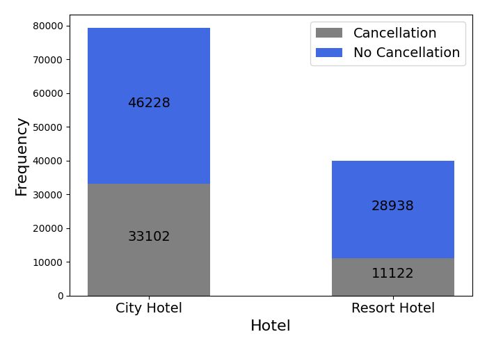
Figure 1. Cancellation condition of different hotels.

Despite the differences mentioned above, if we choose only one hotel for our cancellation prediction research, the results might have low generalization ability. Therefore, to maintain the possibility that the results can adapt to more hotels and diverse occasions, neither of the two hotels is excluded from this research.

2.3.Data cleaning and feature engineering

From the variable types we summarized above, it is obvious that some variables have wrong or inappropriate types. For example, children, agent, and company are float, but children should be integer and the other two should be object. These variables are transited to their proper types.

Table 2 summarizes the columns that have missing values. Children only has 4 values missing, which is understandable considering the loss of data during both the put-in process and transmitting process. The mode of this variable is put in to fill the blanks. As for country, agent, and company, a more significant number of values are missing. It is impossible to delete such a large number of observations from the dataset, or to fill in the blanks by any particular value. Considering the practical meaning of the three values, we find out that the information represented by these variables are not strictly required when making reservations. Some customers may be unwilling to register their countries. And bookings can be made by individual instead of through agent or company. Therefore, the missing values in country column are replaced by ‘unknown’, those in agent column are replaced by ‘NoAgent’, and those in company column replaced by ‘NoCompany’.

Table 2. Number of missing values of selected variables.

The summary statistics for most numerical variables is revealed by Table 3. Variables like cancellation status and year of the reservation are not listed here, because their potential noise cannot be detected by this statistic calculation.

Some abnormalities are found from this summary. ADR, the average amount a guest pays for a room per day, should be a positive value, yet its minimum value is -6.38. Concerning that there are 1960 negative adr values, we replace them by the medium of adr column to avoid discharging too many observations. The minimum value of adults is 0. Because there are only 403 lines with 0 adult, these lines are removed. These abnormal and counterintuitive information may be caused by data entry error.

Table 3. Description of selected numerical variables.

Next, the arrival year, month, and day of the month are combined together to form a complete time variable, named ‘day_of_year’. This variable allows the analysis of time on an accurate level, and can represent the seasonal change of hotel demand. Then, all the redundant variables are removed. They are redundant either because they cause data leakage or because they are private information. Deleting the former can save the dataset from the ruin of these variables, and deleting the latter can confine independent variables on the features of reservations themselves, rather than the personal information of customers. The dropped columns and reasons are shown in Table 4.

Table 4. Variable dropping and specific reasons.

Lastly, all the categorical variables are encoded through dummy encoding. Dummy encoding transforms k discrete features to k-1 binary features. Compared with one-hot encoding that reconstructs k binary features, dummy encoding solves the problem of inter-feature linear relationships.

Now the processed dataset has 118987 observations with 907 features in total. Our goal is to apply different machine learning techniques to predict whether a booking would be cancelled or not based on the processed dataset.

3.Methodologies

3.1.Tools and techniques employed

These data manipulation and machine learning tools are utilized for analysis and modeling of the dataset:

• Python and Data Libraries: In the processes of data understanding and cleaning, Python is the major coding language. Some convenient libraries such as Pandas, NumPy, and Matplotlib are used to analyze and present the large dataset.

efficiently.

• Machine Learning and Deep Learning Frameworks: We employed Scikit-learn for traditional

machine learning models, and deep learning frameworks like TensorFlow for building advanced neural network.

3.2.Hyperparameter tuning

In most machine learning models, there are some parameters that can be settled in advance by people, and that can affect the performance of models. These parameters, named hyperparameter, are searched by GridSearchCV of Scikit-learn in this research. Being offered a grid consists of several parameters and their alternative values, GridSearchCV can find the best permutation among them. All the classical models in this research are tuned more than one time, so as to get more effective and accurate parameters.

To evaluate the performance of every set of parameters, F1-score is used, for it suits imbalanced dataset better than other scores.

3.3.Cross validation

The splitting method of training and test sets can affect the performance of models. Moreover, splitting the data into to sets means that the data is not sufficiently harnessed. To deal with these two problems, cross validation is utilized. The data is shuffled, and then split into five pieces, each piece serving as test set once. Cross validation verifies the stability of the model results, and when used in hyperparameter tuning, guarantees the right choice of parameters.

3.4.Classical models

Since the target of this research is essentially a binary classification question, most classical models are suitable here.

3.4.1.Decision Tree

The Decision Tree is a series of decisions organized in the shape of a tree, i.e., it starts from major and basic decisions but expands them into many minor decisions. In this way, the complicated problem is broken down into a bunch of subsets, and the orderless data is built into a model. An advantage of decision tree is its interpretability, since its major and minor decision can be easily understood as the importance of different features.

Package: sklearn.tree.DcisionTreeClassifier

3.4.2.Random Forest

Random Forest is an ensemble learning method that uses bagging (Bootstrap aggregating). Each time, with replacement, it randomly chooses k observations from the original data to form a subset. It then uses these subsets to build decision tree models, which are its estimators. In classification questions, the final result is the choice of most of the decision tree models. Ensemble learning can decrease overfitting problem and increase the robustness of each estimator, so random forest usually has better predicting ability than decision tree.

Package: sklearn.ensemble.RandomForestClassifier

3.4.3.XGBoost

XGBoost is also an ensemble learning method, yet unlike random forest, it uses boosting algorithm, which means the trees would pay more attention to the wrongly classified samples of the last tree. It has the same basic idea as Gradient Boosting Decision Tree, but it optimizes GBDT in many ways. Compared with GBDT, XGBoost is more accurate, flexible; it reduces overfitting problem, and supports parallel processing.

Package: xgboost.XGBoostClassfier

3.4.4.Logistic Regression

Logistic Regression is a general linear regression analysis model. It uses a streamline to build its model, and map the continuous result into multiple categories. Essentially, it divides the data with a line, a plane, or a hyperplane. It uses sigmoid function to map every set of data into a number between 0 and 1. When the number is larger than 0.5, it is then regarded as belonging to class 1, otherwise it is regarded to be in class 0. It is widely used in many fields due to its simple structure, clear meaning, and easy realization.

Package: sklearn.linear_model.LogisticRegression

3.4.5.MLP

MLP, or artificial neural network, can be divided into input level, implication level, and output level. The input level receives data as neurons. The implication levels extract linear combination from the neurons and get the parameters. The output level uses a process similar to logistic regression to map data into different classes. MLP belongs to Feedforward Neural Network, a basic and common neural network model in deep learning.

Package: sklearn.neural_network.MLPClassifier

3.5.Feature selection

In order to prepare for the building of neural network models, Lasso and PCA are used to select important and informative features from the original 907 features. Firstly, Lasso feature selection method compresses feature coefficients through L1 regularization, which is easy to create sparse weight, to achieve feature selection and dimensionality reduction. After Lasso, the number of features decreased from 907 to 745.

Then, PCA is employed. PCA maps high-dimensional data to a low dimensional space through linear transformation, and maximized the projection variance to ensure that as much information as possible is retained in the reduced space of the original data. In this way, PCA helps simplify the data structure, reduce dimensions, and improve analysis efficiency.

For the choice of the best number of features, we used elbow method and plotted the cumulative explained variance. As is shown in the following Figure, the inflection of the curve is about 700 features, so 700 is selected for the final number of features.

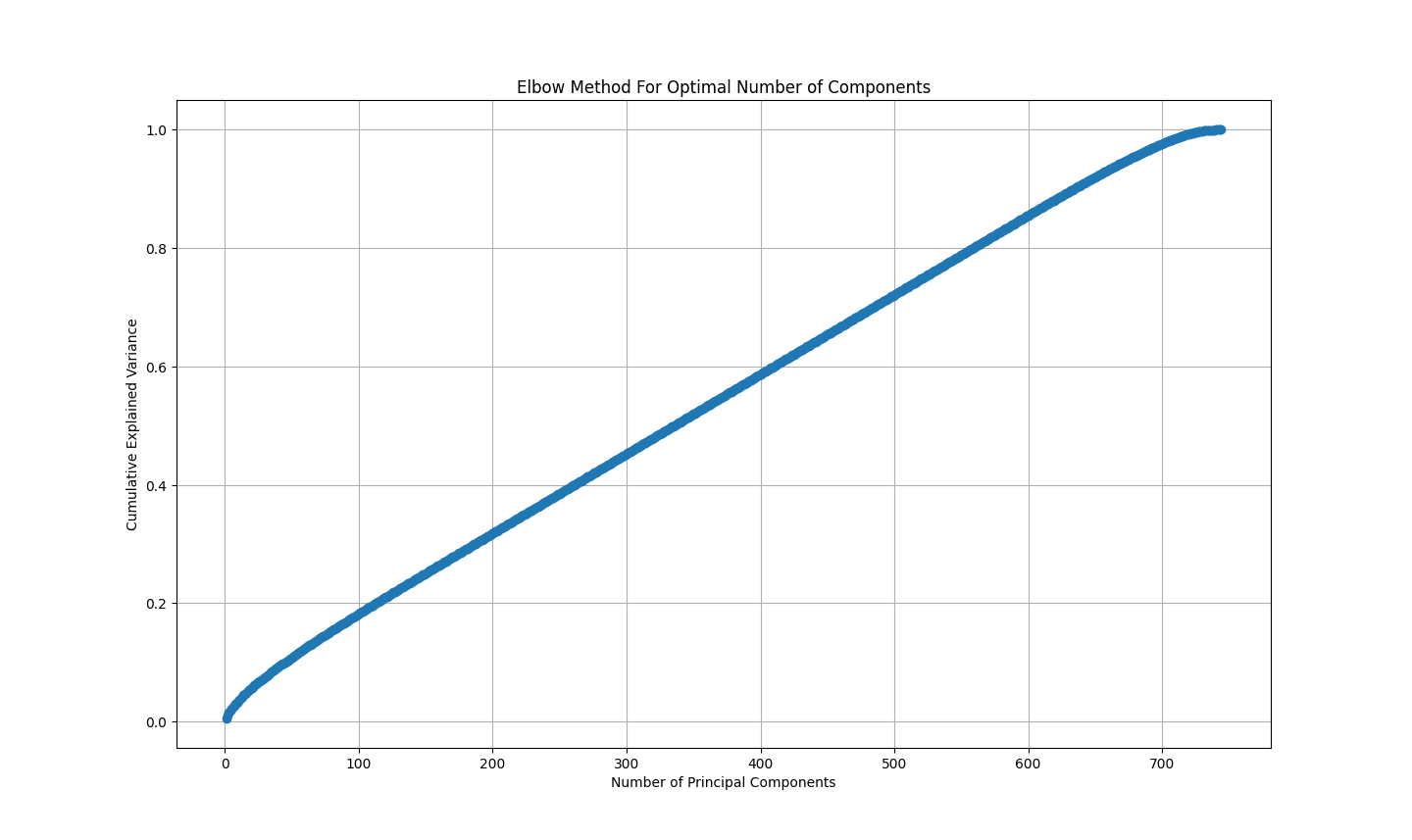
Figure 2. Elbow method for optimal number of components.

3.6.Neural network models

Different from classical models, the neural network models we adopted, namely, CNN, DNN, and LSTM, are all built based on the dataset after feature selection process.

3.6.1.CNN

CNN consists of input layer, convolutional layer, activation function layer, pooling layer, and fully connected layer. It extracts local features of data through convolutional kernels, processes them through activation functions and pooling layers, and outputs classification results through fully connected layers. It has translational invariance and robustness, which can effectively reduce the number of parameters and improve the model's generalization ability.

3.6.2.LSTM

LSTM consists of input gate, forget gate, output gate, and cell state. It controls the inflow and outflow of information through gating mechanisms, and build models based on long-term dependencies. It can process sequential data, have memory and forgetting functions, and is suitable for processing temporal data such as text and speech.

3.6.3.DNN

DNN consists of an input layer, multiple hidden layers, and an output layer, with each layer containing multiple neurons. It automatically extracts data features and approximates complex functions through nonlinear transformations in multiple layers. It has strong fitting ability, feature learning ability, and transferability.

4.Results and discussion

4.1.Model evaluation criteria

To evaluate the performance of models more thoroughly and comprehensively, several evaluation methods are adopted. The score of accuracy, precision (class 1), recall (class 1), F1-score (class 1), and AUC (class 1) are all computed. Accuracy is regarded as the most important and convincing criterion, for it is the most direct pursuit of hotels. Yet other criteria offer their own interpretation of models. The meaning of evaluation methods are as follows.

•Accuracy: The proportion of correctly classified samples to the total number of samples.

•Precision: The proportion of true class 1 samples to the total number of predicted class 1 samples.

•Recall: The proportion of true class 1 samples to the total number of class 1 samples.

•F1-score: A weighted average of precision and recall.

•AUC: The area under ROC curve. The horizontal axis of the ROC curve is FPR (False Positive Rate), and the vertical axis is TPR (True Positive Rate), i.e., recall. ROC illustrates the trade-off between the two axes at various threshold settings. The larger the area is, the finer the performance is.

4.2.Decision tree

4.2.1.Hyperparameter tuning

Class weight, criterion, max depth, min samples leaf, and min samples split are selected as the parameters to be tuned. Parameters are changed and tuned for several rounds to get an optimized result. The meanings of these parameters are shown as follows.

•Class weight: the weight of cancelled and not-cancelled data in model training.

•Criterion: The standard of splitting the nodes and reduce the level of chaos in the dataset.

•Max depth: The max depth of the tree.

•Min samples leaf: When splitting a node, if the node after splitting contains leaves smaller than this number, the splitting process will stop

•Min samples split: When splitting a node, if the node itself contains leaves smaller than this number, the splitting process will stop

As a result, the optimal hyperparameters are:

•class_weight: {0: 1, 1: 2}

•criterion: gini

•max_depth: 20

•min_samples_leaf: 1

•min_samples_split: 2

4.2.2.Model performance

Confusion matrix provides a visual representation of the true positive, true negative, false positive, and false negative predictions. Based on these four types of predictions, accuracy, precision, recall, and F1-score are generated. The ROC curve is plotted to offer a direct revealing of its shape and its area under curve.

Figure 3. Model performance of Decision Tree

The accuracy score of 0.8644 suggests that the model correctly predicts the hotel cancellation approximately 86% of the time. The precision score for class 1 (cancelled) is 0.7835 and the recall score for class 1 is 0.8762. The F1 score for class 1 of 0.8273 indicates a good balance between precision and recall, highlighting the model’s effectiveness in distinguishing between cancelled and not-cancelled cases. The AUC score for class 1 of 0.9047 is way larger than 0.5 score of a random classifier, suggesting that the model does not perform out of randomness and coincidence.

4.3.Random forest

4.3.1.Hyperparameter tuning

Initially, class weight, n estimators, criterion, min samples split, min samples leaf, and max depth are selected as parameters to be tuned. Yet it is found that a confinement of max depth would strongly damage the performance of random forest, max depth is then removed, with the rest continuing the grid search. Parameters are changed and tuned for several times to be more accurate. For example, in the last round, the number of estimators is grid searched in a range of 10

Since random forest is an ensemble of multiple decision trees, their commonly tuned parameters are also similar. The only different parameter, n estimator, means the number of trees generated in random forest model.

As a result, the optimal hyperparameters are:

•class_weight: {0: 1, 1: 3}

•n_estimators: 120

•criterion: entropy

•min_samples_leaf: 1

•min_samples_split: 6

4.3.2.Model performance

In confusion matrix, true positive and true negative predictions largely outnumber the rest two, indicating the reliability in the prediction of the model. Though there are some False Positives and False Negatives, the model is doing a good job of minimizing them. The ROC curve is close to the top-left corner, suggesting that this model has excellent performance.

Figure 4. Model performance of Random Forest

The accuracy score is 0.8913. The precision is 84.47%, which means that approximately 84% of the bookings that the model predicted as canceled were actually canceled. The recall is 86.61%, which means that the model correctly identified approximately 87% of the actual cancellations. The F1-score is 85.53%. The AUC is 95.96%, which means that the model has a very good discriminative power between the two classes.

Compared to the Decision Tree (DT) model, the Random Forest (RF) model shows a significant improvement in all the performance metrics, particularly in reducing the number of False Positives. This indicates that the Random Forest model is better at balancing the trade-off between Precision and Recall, leading to a higher F1-score. Considering that random forest is a combination of decision trees, this result is quite understandable.

4.4.XGBoost

4.4.1.Hyperparameter tuning

Gamma, n_estimators, learning_rate, max_depth, subsample, cosample_bytree, and scale_pos_weight are selected as the parameters to be tuned. Some parameters, such as subsample and colsample_bytree, have limited range of typical value, and are thus easier to tune. For other parameters like n_estimators, many trials were made to find the optimal number. The meanings of these parameters are shown as follows.

•gamma: The minimum required descent value of the loss function for node splitting. Larger value of gamma makes the model more conservative.

•learning_rate: The contribution of every estimator.

•max_depth: The max depth of the tree.

•subsample: The proportion of trees randomly sampled for each estimator.

•cosample_bytree: The proportion of columns (features) randomly sampled for each tree.

•scale_pos_weight: For balancing the samples and making the algorithm to converge faster. In the grid we set two candidate numbers: 1 and (y_train == 0).sum() / (y_train == 1).sum().

As a result, the optimal hyperparameters are:

•gamma: 0.2

•learning_rate: 0.1

•max_depth: 10

•subsample: 0.8

•cosample_bytree: 0.7

•scale_pos_weight: 1.6971834976765272

4.4.2.Model performance

The accuracy score of 0.8881 suggests that the model correctly predicts the hotel cancellation approximately 89% of the time. This accuracy score is slightly lower than random forest. The precision score of 0.8293, the recall score of 0.8793, and the F1 score of 0.8536 are also lower than random forest. However, the AUC is 96.05%, which means it enhances about 1% from the last model, indicating that XGBoost is still quite competent at classification.

Figure 5. Model performance of XGBoost

The confusion matrix mainly differs from that of random forest in false positive. It can be inferred that the higher number of false positive predictions negatively influences the performance of XGBoost.

4.5.Logistic Regression

4.5.1.Hyperparameter tuning

Among the parameters of logistic regression, max_iter is tested in a most detailed way, ranging from 50 to 200. From Figure 5, it can be seen that the accuracy of 50 and 75 times of iteration is relatively low, and starting from the 100^th iteration, the performance of the model stops improving. This reveals that for this logistic regression, some of the default values are already the optimized value.

Figure 6. Effect of max_iter on Logistic Regression performance.

The meanings the other tuned parameters are as follows.

•penalty: The norm that penalty term follows. Parameters to be chosen are l1 and l2.

•c: The reciprocal of the regularization coefficient. It controls the strength of regularization. The less the value is, the stronger the regularization is.

•solver: The parameter to control the process of solvation, including the velocity, accuracy, and stability of question solving. In logistic regression, the parameter to be selected are newton-cg, lbfgs, liblinear, sag, and saga. It should be noted that some of them can only be lined up with l2 penalty.

After grid search, however, most of the optimized parameters are only the default parameters, the only difference is solver, which changed from liblinear to newton-cg.

4.5.2.Model performance

From Figure 5, it can be seen that logistic regression has relatively higher false positive predictions.

Figure 7. Model performance of Logistic Regression

The recall of 84.39% and the AUC of 90.99% are fairly good. Yet the precision is 71.49% and the F1-score is 77.41%. So, compared with former models, the precision and F1-score are low, both scoring only more than 70%. This might be the reason of the accuracy of 81.74%, as a weakness in forecasting those cancelled cases can negatively influence the accuracy of model to some extent.

4.6.MLP

4.6.1.Hyperparameter tuning

The choice of parameters contains some background information. For solver, as lbfgs has better effect on small datasets, it is not included in the grid. For activation, softmax suits multi classification problems better, so the grid only contains logistic and ReLU. Also hidden_layer_sizes is tuned. The meanings of the parameters are shown as follows.

•solver: Solver for weight optimization

•activation: Types of activation functions for neurons. They are nonlinear functions, for nonlinearity can improve the expressive power of the model

•hidden_layer_sizes: The number of hidden layers and neurons can determine the complexity and capacity of MLP

As a result, the optimal hyperparameters are:

•solver: adam

•activation: logistic

•hidden_layer_sizes: (100,100)

4.6.2.Model performance

Figure 8. Model performance of MLP

The accuracy is 84.27%. MLP does particularly well in avoiding false positive predictions, and thus its precision reaches 87.83%. In addition, the recall is 66.84%, the F1-score is 75.91%, and the AUC is 93.06%. However, the confusion matrix shows that MLP makes more false negative predictions compared with other models. It can be inferred that this model is relatively conservative.

4.7.LSTM

4.7.1.Model building

We used Keras library to build a simple sequence model (Sequential), which includes an LSTM layer (64 units, ReLU activation function) for processing time series data and a fully connected layer (Sigmoid activation function) for binary classification. The model is compiled using Adam optimizer and binary cross entropy loss function, and its accuracy is evaluated.

4.7.2.Model performance

In the end, the model reached the accuracy of about 99.63%, indicating that it excellently grasped the features of data and is able to make precise predictions.

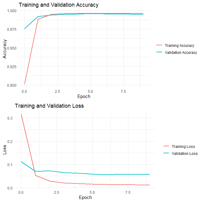
Figure 9. The change of training loss and validation accuracy, training and validation accuracy in different epochs.

The training and validation accuracy and loss curves are shown in the figures above. These curves provide insights into the model’s learning process over the 10 epochs.

• Training and Validation Accuracy: The training accuracy goes up quickly in Epoch 1, indicating that the model is learning and improving its performance swiftly on the training data. After that, the training accuracy remains relatively steadily above 99%, with only minor changes. This shows that LSTM learns this data so fast that most new information is studied in Epoch 1.

• Training and Validation Loss: The training loss accordingly decreases rapidly in Epoch 1, which is expected as the model learns to minimize the loss function. After that, both losses descend slowly. Starting from epoch 1, the validation loss is always higher than training loss, indicating that the performance on training data is better than that on validation data.

4.8.CNN

4.8.1.Model building

A simple one-dimensional convolutional neural network (1D CNN) model is built for processing sequential data. The model includes a Conv1D layer for feature extraction, a MaxPooling1D layer for dimensionality reduction, a Flatten layer for flattening multidimensional data, and finally two fully connected layers, Dense, to output a sigmoid activated prediction value.

4.8.2.Model performance

The accuracy of CNN reached 99.79% in the end.

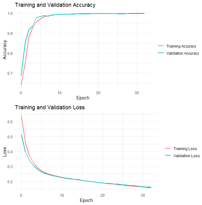
Figure 10. The change of training loss and validation accuracy, training and validation accuracy in different epochs.

The training and validation accuracy and loss curves are shown in the figures above, providing insights into the model’s learning process over the 33 epochs.

• Training and Validation Accuracy: The training accuracy grows quickly in the first 5 epochs, and remains very close to 1 in latter epochs, with minor improvement. Though the validation accuracy grows up turbulently, the training accuracy grows steadily.

• Training and Validation Loss: The training loss keeps decreasing over the epochs, with a turning point at about epoch 5. The model’s performance on the validation set perfectly matches the training set, suggesting a strong performance of the model.

4.9.DNN

4.9.1.Model building

A simple neural network model was constructed using TensorFlow and Keras, consisting of three fully connected layers (Dense layers). The first Dense layer has 64 neurons, uses ReLU activation function, and receives input data. The second Dense layer also has 64 neurons and uses the ReLU activation function. The third Dense layer is the output layer with only one neuron, using the sigmoid activation function for binary classification tasks. The optimizer, loss function, and evaluation method are same as LSTM, namely, Adam, binary cross entropy, and accuracy.

4.9.2.Model performance

The accuracy of DNN reached 99.87%, indicating that it can almost correctly classify all the booking records.

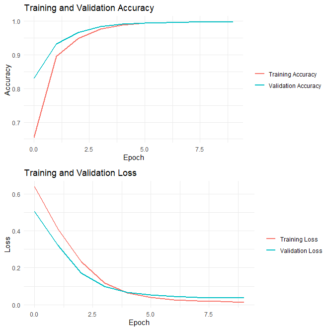
Figure 11. The change of training loss and validation accuracy, training and validation accuracy in different epochs.

The training and validation accuracy and loss curves are shown in the figures above, providing insights into the model’s learning process over the 10 epochs.

• Training and Validation Accuracy: The training accuracy shows a general upward trend, especially in the first 5 epochs. Though in the latter 5 epochs, the growing rate of accuracy slows down, the good thing is that the validation accuracy does not decrease, and the training and validation accuracies are similar, suggesting that the model is not overfitting to the training data.

• Training and Validation Loss: The training loss keeps decreasing over the epochs. To be specific, there is a turning point at epoch 4, before which the loss decreases relatively swiftly, while after which its decrease rate apparently slows down. The model’s performance on the validation set is slightly worse the training set, suggesting that it may not generalize well to all unseen data.

4.10.Model comparison and analysis

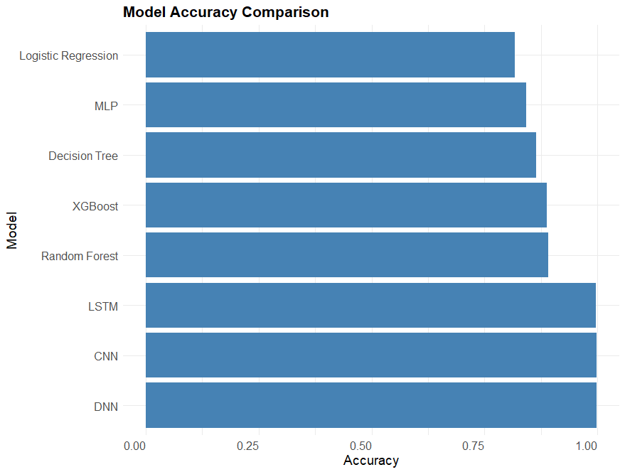
Figure 12. Model accuracy comparison.

The bar plot summarizes the accuracy of all models. In classical models, logistic regression performs worst, and random forest is the best. This reveals the advantage of ensemble learning method, and in this particular case, bagging is more effective than boosting. The neural network models score remarkably better than classical models. However, for the dataset for neural network models has gone through feature selection process including Lasso and PCA, it is inferred that the feature selection is virtually the biggest contributor to these results, rather than neural network models themselves. This indicates that feature selection has special importance in this dataset.

5.Conclusion

In this study, we used machine learning to deal with PMS data from hotels, in the hope of forecasting hotel booking cancellations. The process includes data cleaning, feature engineering, feature selection, and model building, which should be a standard and rigorous process of dealing with a large dataset. Several statistical techniques were employed to handle missing values, counterintuitive values, and a posterior information that largely influence the model prediction. The processed dataset has not only high quality, but also meaningful and interpretable features. Feature selection and dimensionality reduction methods, including PCA and Lasso, were utilized to identify the most predictive features, and thus prepare for the more rapid establishment of neural network models.

A comprehensive set of machine learning and deep learning models were implemented, including Logistic Regression, Decision Tree, Random Forest, XGBoost, MLP, CNN, DNN, and LSTM. Each model demonstrated unique strengths: Logistic Regression provided simplicity and interpretability; Random Forest offered robust predictions with insights into feature importance; CNN captured spatial and sequential patterns in data; LSTM effectively modeled long-term dependencies in time-series data. The results are impressing, with the accuracy of all models over 80%, and that of the neural network models nearly 100%. This indicates that the models can successfully predict the cancellation of several hotels, and that there is a similar mode of cancellation among hotels.

This research also has some limitations in spite of its achievements. In feature engineering process, some hidden relationships of data might be discovered, and better ways of transforming data might be discovered and employed. In model building process, there are some intrinsic problems of models. For example, deep learning models, especially LSTM networks, require a large amount of computational resource, which may limit their practicality. The complexity of models such as DNN makes them difficult to explain and requires additional tools to understand the decision-making process. The performance of the model is affected by the quality and quantity of data. Insufficient or noisy data may hinder the model's ability to learn meaningful patterns.

Future works can be done based on data of longer timeline and from more hotels, with more integrality and accuracy. In addition, when processing the original data, more novel and effective feature engineering methods can be used on the basis of richer experience of hotel management. As PCA has an extraordinarily positive influence on the final result, more ways of feature selection can be experimented. In terms of model building, more advanced models can be wielded, and the hyperparameters can be tuned more meticulously.

In summary, this study uses deep learning to address the issue of predicting hotel reservation cancellations. The methods and advancements mentioned above provide deeper insights and more accurate predictions, paving the way for future innovation and applications.

References

[1]. Zhu, X. (2022). Qualitative research on the life meaning experience of adolescent depression patients with non-suicidal self-injury. Zhejiang University of Traditional Chinese Medicine.
[2]. Hazarika, S., Li, H., Wang, K. C., Shen, H. W., & Chou, C. S. (2019). NNVA: Neural network assisted visual analysis of yeast cell polarization simulation. IEEE Transactions on Visualization and Computer Graphics, 26(1), 34-44.
[3]. Grimaldo, A. I., & Novak, J. (2020). Combining machine learning with visual analytics for explainable forecasting of energy demand in prosumer scenarios. Procedia Computer Science, 175, 525-532.
[4]. Wang, Q., Chen, Z., Wang, Y., & Qu, H. (2021). A survey on ML4VIS: Applying machine learning advances to data visualization. IEEE Transactions on Visualization and Computer Graphics, 28(12), 5134-5153.
[5]. Ndiaye, B. M., Balde, M. A., & Seck, D. (2020). Visualization and machine learning for forecasting of COVID-19 in Senegal. arXiv preprint arXiv:2008.03135.
[6]. Zheng, G., Zhang, F., Zheng, Z., Xiang, Y., Yuan, N. J., Xie, X., & Li, Z. (2018, April). DRN: A deep reinforcement learning framework for news recommendation. In Proceedings of the 2018 World Wide Web Conference (pp. 167-176).
[7]. Smart, S., Wu, K., & Szafir, D. A. (2019). Color crafting: Automating the construction of designer quality color ramps. IEEE Transactions on Visualization and Computer Graphics, 26(1), 1215-1225.
[8]. Wu, A., Tong, W., Dwyer, T., Lee, B., Isenberg, P., & Qu, H. (2020). Mobilevisfixer: Tailoring web visualizations for mobile phones leveraging an explainable reinforcement learning framework. IEEE Transactions on Visualization and Computer Graphics, 27(2), 464-474.
[9]. Taigman, Y., Yang, M., Ranzato, M. A., & Wolf, L. (2014). Deepface: Closing the gap to human-level performance in face verification. In Proceedings of the IEEE Conference on Computer Vision and Pattern Recognition (pp. 1701-1708).
[10]. Ribeiro, M. T., Singh, S., & Guestrin, C. (2016, August). "Why should I trust you?" Explaining the predictions of any classifier. In Proceedings of the 22nd ACM SIGKDD International Conference on Knowledge Discovery and Data Mining (pp. 1135-1144).
[11]. Gui, J., Sun, Z., Wen, Y., Tao, D., & Ye, J. (2021). A review on generative adversarial networks: Algorithms, theory, and applications. IEEE Transactions on Knowledge and Data Engineering, 35(4), 3313-3332.
[12]. Krizhevsky, A., Sutskever, I., & Hinton, G. E. (2012). Imagenet classification with deep convolutional neural networks. Advances in Neural Information Processing Systems, 25.
[13]. Chatzimparmpas, A., Martins, R. M., Jusufi, I., & Kerren, A. (2020). A survey of surveys on the use of visualization for interpreting machine learning models. Information Visualization, 19(3), 207-233.
[14]. Alharbi, M., & Laramee, R. S. (2018, September). SoS TextVis: A Survey of Surveys on Text Visualization. In CGVC (pp. 143-152).
[15]. Caicedo-Torres, W., & Payares, F. (2016). A machine learning model for occupancy rates and demand forecasting in the hospitality industry. In Advances in Artificial Intelligence-IBERAMIA 2016: 15th Ibero-American Conference on AI, San José, Costa Rica, November 23-25, 2016, Proceedings 15 (pp. 201-211). Springer International Publishing.
[16]. Antonio, N., De Almeida, A., & Nunes, L. (2017). Predicting hotel booking cancellations to decrease uncertainty and increase revenue. Tourism & Management Studies, 13(2), 25-39.
[17]. Antonio, N., de Almeida, A., & Nunes, L. (2017, December). Predicting hotel bookings cancellation with a machine learning classification model. In 2017 16th IEEE International Conference on Machine Learning and Applications (ICMLA) (pp. 1049-1054). IEEE.
[18]. Satu, M. S., Ahammed, K., & Abedin, M. Z. (2020, December). Performance analysis of machine learning techniques to predict hotel booking cancellations in hospitality industry. In 2020 23rd International Conference on Computer and Information Technology (ICCIT) (pp. 1-6). IEEE.
[19]. Adil, M., Ansari, M. F., Alahmadi, A., Wu, J. Z., & Chakrabortty, R. K. (2021). Solving the problem of class imbalance in the prediction of hotel cancelations: A hybridized machine learning approach. Processes, 9(10), 1713.
[20]. Sánchez-Medina, A. J., & Eleazar, C. (2020). Using machine learning and big data for efficient forecasting of hotel booking cancellations. International Journal of Hospitality Management, 89, 102546.
[21]. Lee, M., Mu, X., & Zhang, Y. (2020). A machine learning approach to improving forecasting accuracy of hotel demand: A comparative analysis of neural networks and traditional models. Issues in Information Systems, 21(1).
Cite this article
Sun,J. (2025). Hotel booking cancellation and machine learning. Advances in Engineering Innovation,15,45-62.
Data availability
The datasets used and/or analyzed during the current study will be available from the authors upon reasonable request.
Disclaimer/Publisher's Note
The statements, opinions and data contained in all publications are solely those of the individual author(s) and contributor(s) and not of EWA Publishing and/or the editor(s). EWA Publishing and/or the editor(s) disclaim responsibility for any injury to people or property resulting from any ideas, methods, instructions or products referred to in the content.
About volume
Journal:Advances in Engineering Innovation
© 2024 by the author(s). Licensee EWA Publishing, Oxford, UK. This article is an open access article distributed under the terms and
conditions of the Creative Commons Attribution (CC BY) license. Authors who
publish this series agree to the following terms:
1. Authors retain copyright and grant the series right of first publication with the work simultaneously licensed under a Creative Commons
Attribution License that allows others to share the work with an acknowledgment of the work's authorship and initial publication in this
series.
2. Authors are able to enter into separate, additional contractual arrangements for the non-exclusive distribution of the series's published
version of the work (e.g., post it to an institutional repository or publish it in a book), with an acknowledgment of its initial
publication in this series.
3. Authors are permitted and encouraged to post their work online (e.g., in institutional repositories or on their website) prior to and
during the submission process, as it can lead to productive exchanges, as well as earlier and greater citation of published work (See
Open access policy for details).