1. Introduction

Single-particle tracking is widely used in microscopy applications to study the dynamic behavior of biomolecules, cells, and nanomaterials. By tracking the changes of particles in both time and space, researchers can gain deep insights into the motion patterns, interactions, and behavior of particles in complex environments. This technique holds significant value in various fields, including cell biology, physics, and chemistry. However, when observing particles under a microscope, the recorded particle trajectories are often subject to significant noise interference due to various factors related to the equipment, environment, and imaging system [1]. A major source of such interference is jitter, which arises from minor vibrations in the microscope, changes in the external environment, or instability in the imaging system. This jitter causes fluctuations in particle positions, making the true motion trajectory of the particle unclear, which in turn affects the accuracy of the data and can undermine the reliability of experimental conclusions.

To overcome this issue, it is essential to remove the irrelevant jitter signals during the post-processing stage to ensure precise measurement of particle motion [2]. Filtering methods are commonly used techniques in particle processing [3-5]. By processing particle trajectories in the frequency domain, a low-pass filter can effectively remove high-frequency noise associated with jitter while preserving the overall trend of particle motion [6]. The core concept of a low-pass filter is that the true motion of the particle typically manifests as low-frequency signals, while jitter tends to exhibit high-frequency components [7]. Therefore, filtering can retain the motion signal while removing the high-frequency noise, resulting in smoother and more accurate velocity estimation and particle trajectories.

Although low-pass filtering methods are theoretically effective at reducing jitter, traditional anti-shake algorithms still have several limitations. Many classical anti-shake algorithms rely on fixed filter designs, such as a constant cutoff frequency or simple smoothing techniques [8]. While these methods can be effective in some cases, they often fail to adapt to the varying jitter characteristics under different experimental conditions. For instance, in complex dynamic systems, particle motion may not only involve simple translation but also rotation, acceleration, and other complex non-linear movements. In such cases, traditional low-pass filtering methods may not effectively distinguish between true motion and noise, resulting in excessive smoothing of the signal and even loss of critical information about the particle’s movement. Additionally, traditional methods often depend on manually set cutoff frequencies, which may lead to over-filtering or under-filtering under different experimental conditions. For example, the frequency range of jitter may vary with experimental setups, and a fixed cutoff frequency may not be suitable for all scenarios. Even when adaptive filtering methods are used, they typically fail to accurately capture the characteristics of the jitter, requiring further manual adjustments and optimization.

To address these issues, this paper proposes a Fourier transform-based particle velocity optimization framework. This framework transforms the particle motion signal from the time domain to the frequency domain through Fourier transform, followed by the application of a low-pass filter for noise removal. Unlike traditional methods, our framework automatically adjusts the filter's cutoff frequency using a numerical optimization algorithm to minimize the error between the particle velocity and the true trajectory, thus adaptively optimizing the filtering effect under varying experimental conditions. Specifically, we adopt a Mean Squared Error (MSE)-based optimization objective, minimizing the error to automatically determine the optimal cutoff frequency, ensuring accurate particle velocity estimation and smooth particle trajectories. Our algorithm offers significant advantages. First, by using Fourier transform, it can precisely identify high-frequency noise components in the particle's motion and effectively eliminate unnecessary interference. Second, the automatic adjustment of the cutoff frequency through numerical optimization avoids the limitations associated with manually set cutoff frequencies, ensuring that the algorithm achieves the optimal filtering effect under different experimental conditions. Finally, our framework not only performs excellently in handling common jitter noise but is also adaptable to nonlinear motion in complex dynamic systems, providing more accurate velocity estimation and particle trajectory reconstruction.

2. Method

2.1. Particle motion coordinate acquisition

The raw video is a grayscale video captured at 60 frames per second with a resolution of 220x220 pixels, and it is in AVI format. To extract particle coordinates from the raw video files, we utilized FIJI software, a distribution of ImageJ. First, the raw video was imported into FIJI, where its built-in particle detection function was employed. By setting an appropriate threshold, particles in each frame were automatically identified. Subsequently, FIJI extracted the center coordinates of the particles in each frame (POSITION_X, POSITION_Y) and saved these coordinates as a CSV file, which served as the foundation for subsequent velocity calculations and filtering processes.

2.2. Data preprocessing and calculation

In this study, the velocity signal was first calculated from the raw position data. For the position coordinate sequence, POSITION_X and POSITION_Y represent the X and Y coordinates at time t, respectively. The velocity was calculated by determining the positional change between adjacent frames, with the frame rate of the current video being 60 FPS, meaning the time interval between each frame is \( T=\frac{1}{60} \) s. The formula for calculating the particle velocity is as follows:

\( v(t)=\frac{\sqrt[]{{(x(t+1)-x(t))^{2}}+{(y(t+1)-y(t))^{2}}}}{T}\ \ \ (1) \)

Here, \( v(t) \) represents the velocity at the time point t, with units of pixels per seconds. Thought preprocessing, we obtained the velocity signal sequence \( v(t) \) from the spital position data, which was then used for subsequent Fourier transform and filtering process.

2.3. Particle velocity optimization framework

In this study, we propose a Fourier transform-based particle velocity optimization framework that improves the accuracy of velocity data by filtering and optimizing the particle trajectories. The framework includes the following main steps: Fourier transform and low-pass filtering, metric calculation, and optimization process. The detailed workflow is shown in Figure 1.

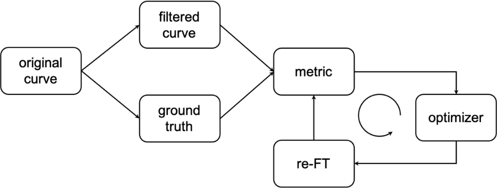
Figure 1. Workflow of the particle velocity optimization framework.

The process begins with the original curve, which undergoes filtering to produce the filtered curve. The ground truth is then used to calculate a metric, and the Fourier transform is applied again (re-FT). Finally, an optimizer refines the results to improve the accuracy of the velocity data.

First, we perform a Fourier transform on the computed velocity signal to convert it from the time domain to the frequency domain. The Fourier transform formula is as follows:

\( \hat{v}(t)=\sum _{t=0}^{N-1}v(t){e^{-i2πft}}\ \ \ (2) \)

Here, \( \hat{v}(t) \) represents the frequency domain representation of the velocity signal, \( f \) is the frequency,and \( N \) is the number of samples of the signal｡In the frequency domain, we apply a low-pass filter to remove high-frequency noise that contains jitter, while retaining the overall trend of the motion. The frequency domain processing rule for the low-pass filter is as follows:

\( {\hat{v}_{filtered}}(t)=\begin{cases} \begin{array}{c} \hat{v}(t), if |f|≤{f_{c}} \\ 0, if|f| \gt {f_{c}} \end{array} \end{cases}\ \ \ (3) \)

Here, \( {f_{c}} \) represents the cutoff frequency. After filtering, only the low-frequency velocity signals are retained, while high-frequency noise is filtered out. Subsequently, the inverse Fourier transform is applied to convert the signal back to the time domain, resulting in the smoothed velocity curve \( {v_{filtered}}(t) \) :

\( {v_{filtered}}(t)=\sum _{f}{\hat{v}_{filtered}}(t){e^{-i2πft}}\ \ \ (4) \)

To evaluate the filtering effect, we calculate the distance between the filtered velocity and the ground truth trajectory, and the error with calculation is shown in Figure 2. \( {v_{gt}}(t) \) represents the velocity signal of the ground truth trajectory. The error metric is based on the Mean Squared Error (MSE), which is used to better reflect the magnitude of the distance:

\( Metric=\frac{1}{N}\sum _{t=0}^{N-1}{({v_{filtered}}(t)-{v_{gt}}(t))^{2}}\ \ \ (5) \)

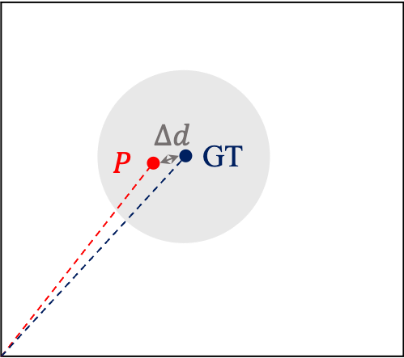
Figure 2. Distance between ground truth and output position.

This figure shows the distance \( △d \) between the ground truth and the output position P. The distance is computed at each time step and used to evaluate the performance of the filtering algorithm.

To automatically optimize the cutoff frequency \( {f_{c}} \) of the low-pass filter, we employ a numerical optimization method. The cutoff frequency is adjusted by minimizing the metric function. The specific optimization objective is as follows:

\( f_{c}^{opt}=arg{ \underset{{f_{c}}}{min}{(Metric({f_{c}}))}}\ \ \ (6) \)

During the optimization process, the initial cutoff frequency is set to \( {f_{c}}=3.0Hz \) .The optimization method for adjusting the cutoff frequency \( {f_{c}} \) is as follows: Starting with an initial setting for \( {f_{c}} \) , the frequency is adjusted randomly by a step size \( ∆f=\frac{{f_{c}}}{10} \) , either increasing or decreasing it. The change in the metric is then observed. If the metric decreases, indicating an improvement, the new \( f_{c}^{new} \) setting is considered valid, and the next adjustment will follow this direction. This iterative process continues until the metric reaches its minimum, ensuring that the optimal \( f_{c}^{opt} \) is found, which minimizes the error between the filtered velocity and the ground truth trajectory.

3. Result

3.1. Video processing and velocity data acquisition

Figure 3 shows the particle trajectory coordinates extracted from the raw video file using the FIJI software. The image on the left represents the raw frame from the video, while the image on the right shows the result after preprocessing using FIJI. The target particle is marked with a red arrow, and the trajectory of the particle is visualized in purple, indicating its movement over time.

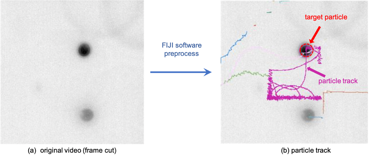
Figure 3. Particle trajectories extracted from raw video using FIJI software.

The left image shows the raw frame, while the right image highlights the particle track after preprocessing, with the target particle and its trajectory labeled.

After extracting the position data from the video, the corresponding velocity information was calculated by determining the changes in particle positions between adjacent frames, and the details were shown in Table 1. This velocity information was then visualized over time, as shown in the lower part of Figure 3. In addition to the velocity magnitude, we also visualized the changes in velocity direction. The upper part of Figure 4 illustrates the particle's movement direction in a schematic form, where different colors represent different directional categories (Left-Down, Right-Down, Right-Up, and Left-Up). The corresponding plot below shows the velocity over time, with each data point colored according to its direction. As can be seen, the particle's velocity direction fluctuates frequently, indicating that the particle undergoes complex motion that changes direction over time.

Table 1. Velocity Statistics of the Particle Over Time

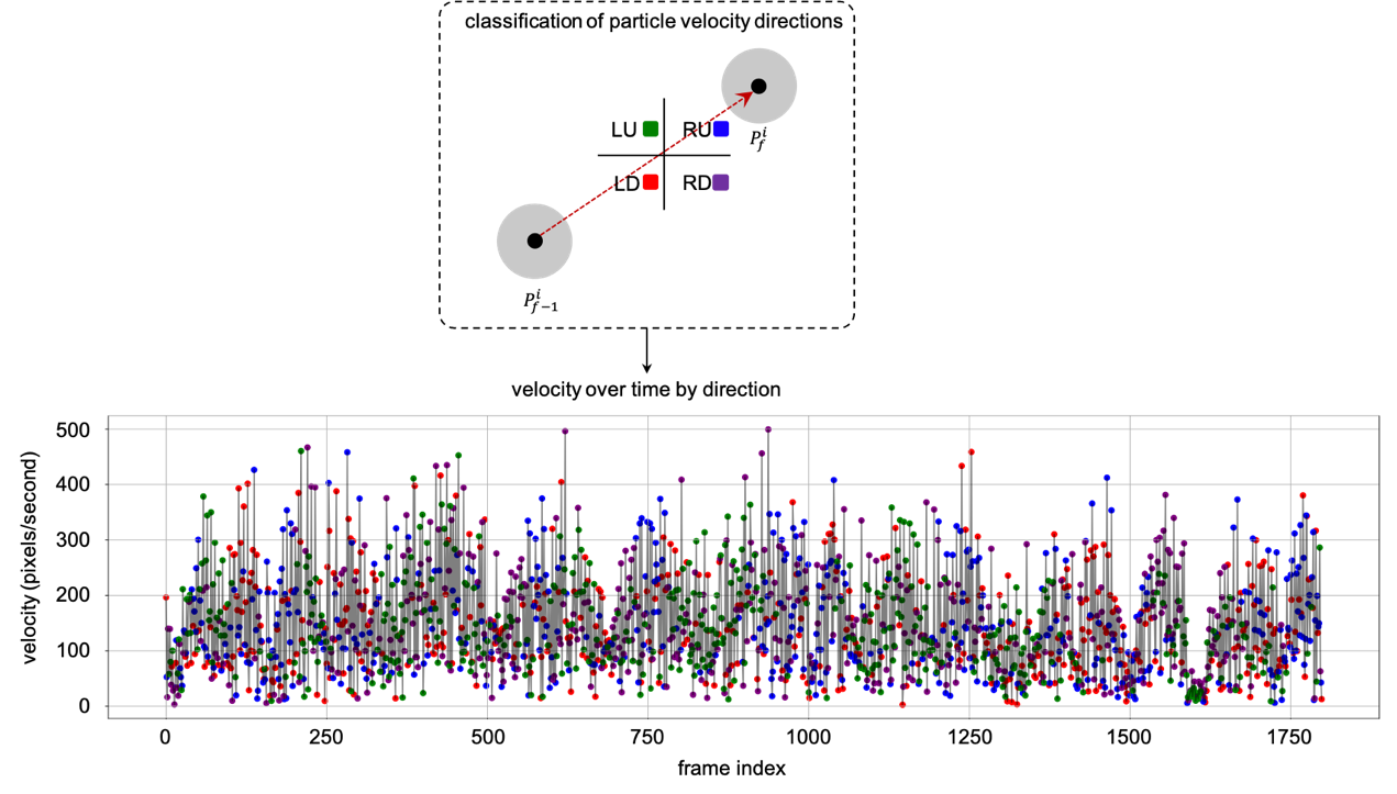
Figure 4. Velocity over time by direction.

3.2. Fourier transform and framework execution

To evaluate the impact of low-pass filtering on the velocity signal, we analyze both the time-domain and frequency-domain representations of the data. Figure 5 presents the velocity signal before and after applying low-pass filters with different cutoff frequencies, while Figure 6 illustrates the corresponding frequency spectra.

Figure 5 displays the velocity signal over time, demonstrating the effects of different low-pass filter settings. The first plot shows the raw velocity signal, which exhibits substantial high-frequency noise due to measurement artifacts and system jitter. The subsequent plots illustrate the filtered velocity signals with cutoff frequencies of 0.5 Hz, 1 Hz, and 3 Hz, respectively.

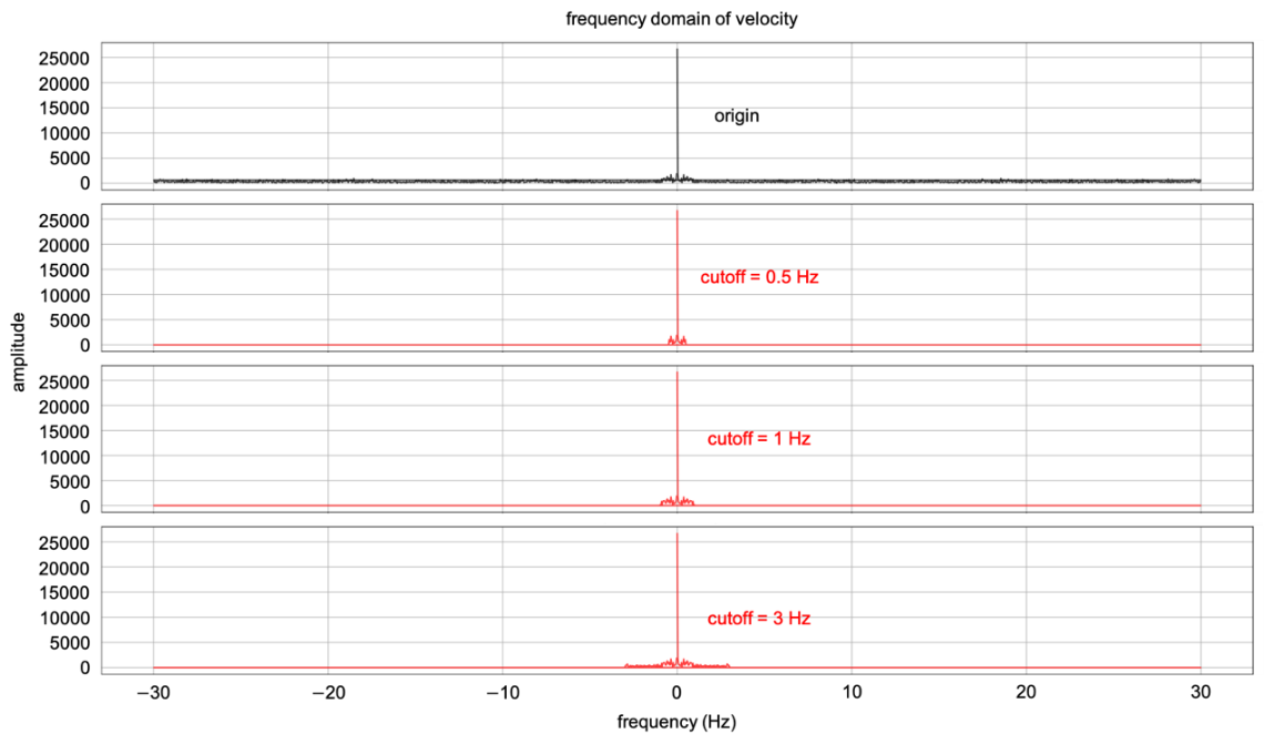
Figure 5. Effect of low-pass filtering on velocity over time

To further examine the filtering effects, Figure 6 presents the Fourier transform of the velocity signal before and after filtering. The first plot shows the unfiltered velocity spectrum, where significant high-frequency noise components are present. The remaining plots display the frequency spectra after applying low-pass filters at 0.5 Hz, 1 Hz, and 3 Hz.

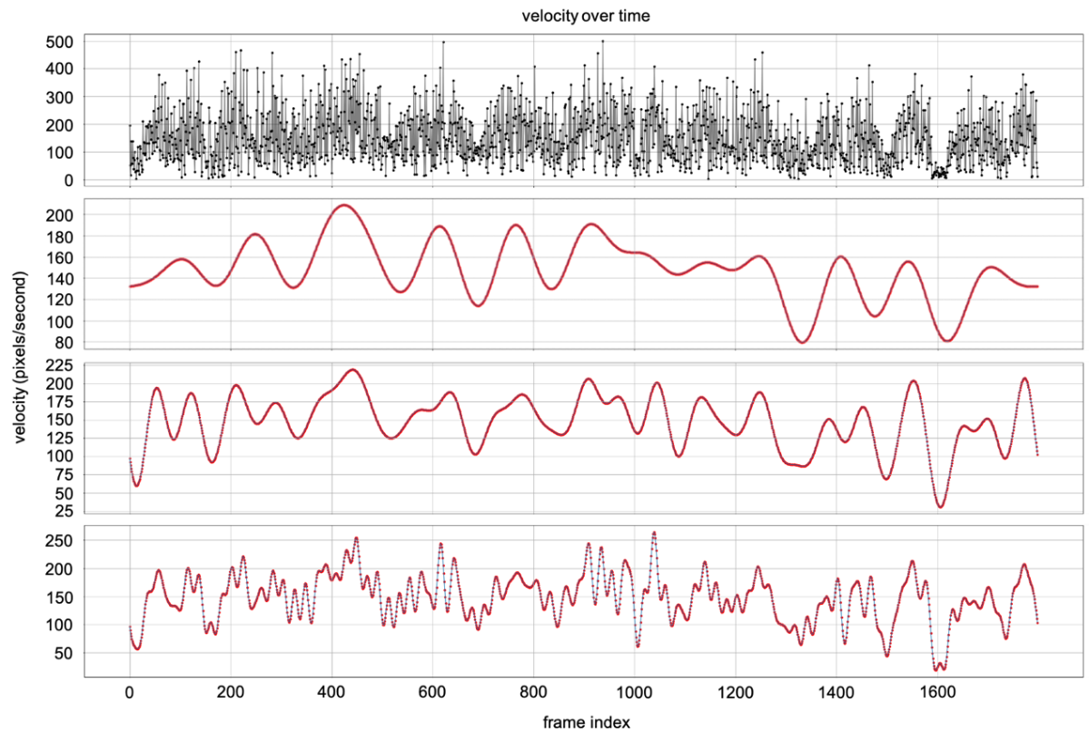
Figure 6. Frequency domain representation of velocity signals with different cutoff frequencies

Building upon the velocity analysis and visualization presented earlier, we now evaluate the effect of varying cutoff frequencies on the performance of the filtering process. When applying our proposed framework, Figure 7 shows the impact of various cutoff frequencies on the normalized metric, which quantifies the error between the filtered velocity signal and the ground truth. The normalized metric decreases as the cutoff frequency reduces, indicating an improvement in the alignment between the filtered velocity signal and the ground truth. At higher cutoff frequencies (e.g., 3 Hz), the metric remains high, suggesting that significant high-frequency noise is retained, which reduces the accuracy of the filtered velocity. As the cutoff frequency decreases, the metric value drops, indicating more effective filtering and better matching with the ground truth. However, the metric value plateaus at around 1 Hz, as marked by the arrow, suggesting that further reducing the cutoff frequency beyond this point leads to diminishing improvements in the accuracy of the velocity signal. This suggests that 1 Hz is near the optimal cutoff frequency, balancing noise reduction and preserving the main features of the particle’s motion.

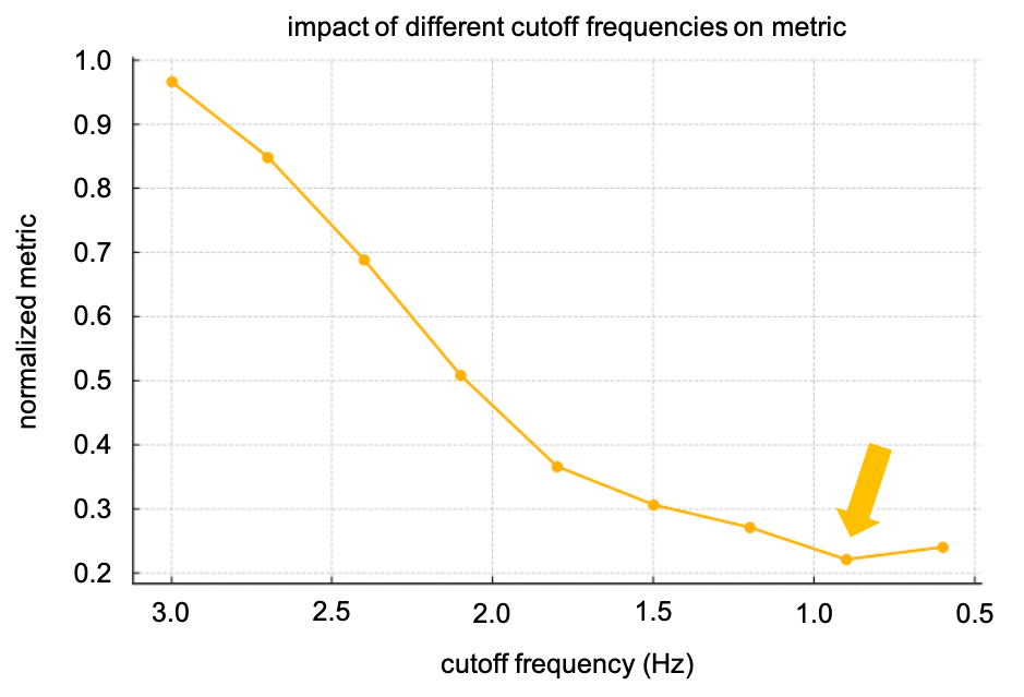
Figure 7. Impact of different cutoff frequencies.

The plot demonstrates how varying the cutoff frequency affects the filtering performance and provides insight into the optimal cutoff frequency for minimizing the error between the filtered signal and the ground truth trajectory.

After the processing of the frame, we got the final particle motion trajectory to remove the jitter. Figure 8 displays the particle trajectory after processing through the proposed filtering framework. The plot shows the filtered trajectory of the particle, where the noise-induced fluctuations in the raw data have been effectively removed. The trajectory is much smoother compared to the original.

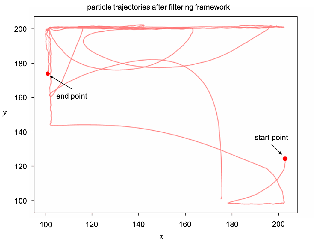
Figure 8. Particle trajectory plot after filtering framework processing.

The red line represents the trajectory of particle motion, from the starting point to the ending point of the motion.

4. Discussion

In this study, we proposed a Fourier transform-based particle velocity optimization framework to improve the accuracy of velocity estimation in single-particle tracking experiments. When tracking particles under a microscope, measurement noise and system jitter introduce high-frequency fluctuations that can obscure the true motion of the particle. To address this issue, we applied a low-pass filtering approach, where the cutoff frequency is optimized through a numerical search method to minimize the discrepancy between the filtered velocity and the ground truth trajectory.

The primary objective of this study was to develop an automated filtering strategy that effectively removes high-frequency noise while preserving the essential motion characteristics of the particle. Unlike conventional filtering techniques that rely on manually set cutoff frequencies, our method dynamically adjusts the cutoff frequency using an optimization process to achieve the best possible filtering performance. Through both time-domain and frequency-domain analyses, we demonstrated how different cutoff frequencies influence the velocity signal and identified an optimal filtering threshold that balances noise reduction and trajectory preservation.

By evaluating the impact of various cutoff frequencies on a metric function, we observed that excessively low cutoff frequencies over-smooth the velocity signal, potentially removing meaningful motion features, while high cutoff frequencies retain unwanted noise. Our optimization approach identified an optimal cutoff frequency (~1 Hz) that minimizes the filtering error, ensuring that the processed velocity signal aligns more closely with the true motion of the particle.

To further evaluate the effect of cutoff frequency on the filtering performance, we also considered the Signal Retention Ratio (SRR) \( P \) as an additional perspective. The SRR provides an insight into how well the signal’s essential components are retained during filtering, by comparing the filtered signal’s amplitude relative to the original signal across different frequencies.

\( P=\frac{{A_{filter}}}{{A_{origional}}}=\frac{\sum _{f \lt t}|Y(f)|}{\sum _{f}|Y(f)|}\ \ \ (7) \)

As shown in Figure 9, SRR was calculated by adjusting the cutoff frequency between 0 Hz and 5 Hz. The plot demonstrates that the SRR increases as the cutoff frequency increases, indicating that more of the original signal is preserved. Notably, the SRR reaches a saturation point near 1 Hz, where the curve flattens, suggesting that beyond this cutoff frequency, further increases in frequency do not significantly improve the retention of useful signal components.

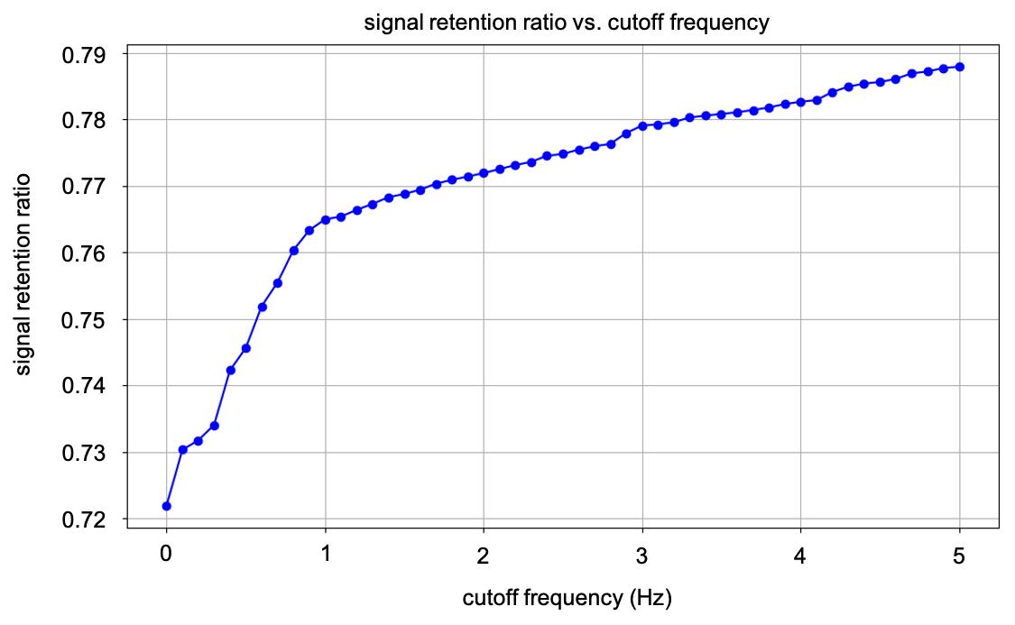
Figure 9. Signal retention ratio vs. cutoff frequency.

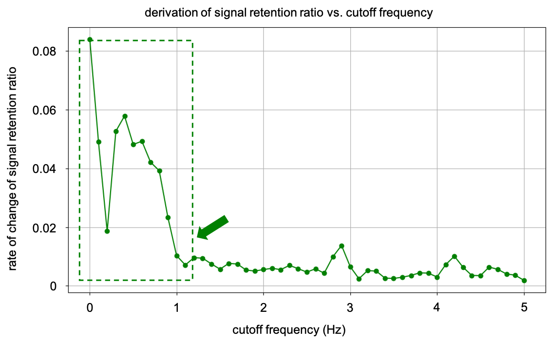
Figure 10. Derivative of signal retention ratio vs. cutoff frequency.

The green dashed box indicates the region that may correspond to the main motion in the low-frequency domain, and the green arrow marks the point of maximum rate of change.

In Figure 10, we further explore the rate of change of SRR by calculating its derivative with respect to cutoff frequency. The plot reveals a sharp increase in the rate of change near 1 Hz, which corresponds to a significant improvement in signal retention at this frequency. This rapid increase indicates that the optimal cutoff frequency for filtering is indeed around 1 Hz, where the filtering process becomes most effective at preserving the essential features of the particle's motion while removing high-frequency noise. These findings align with the results from our Fourier transform-based optimization framework, where the optimal cutoff frequency was also found to be around 1 Hz. Both perspectives — SRR and our filtering framework — point to a similar optimal cutoff frequency, reinforcing the validity of our chosen parameter.

While this study provides valuable insights into optimizing the cutoff frequency for low-pass filtering of particle velocity signals, there are several limitations that should be addressed in future research. Firstly, this study focuses on a single particle, and the analysis is limited to its velocity signal, which restricts the broader applicability of the framework [9]. In real-world applications, multiple particles are often tracked simultaneously, and their interactions or independent motions may vary. Extending the framework to handle multiple particles would enhance its practical utility, especially in complex experimental setups where multiple trajectories need to be analyzed concurrently. Secondly, while the proposed framework allows for adaptive adjustment of the cutoff frequency, it does not yet account for variations in the particle’s motion across different time segments [10]. In future research, the framework could be further refined by incorporating the possibility of dynamically setting different cutoff frequencies based on the varying characteristics of velocity in different time periods.

5. Conclusion

this study presents a Fourier transform-based particle velocity optimization framework that effectively addresses the challenges of high-frequency noise in particle tracking experiments. By optimizing the cutoff frequency of the low-pass filter, the framework offers a method for adaptively reducing noise while preserving the key features of particle motion. The results demonstrate that an optimal cutoff frequency, around 1 Hz, provides the best balance between noise reduction and signal preservation. This approach significantly improves the accuracy of velocity estimation and trajectory reconstruction, providing a valuable tool for researchers in fields such as cell biology, physics, and materials science, where precise particle motion analysis is essential.

References

[1]. Wang, B., Zhang, X. X., Sun, Y. J., Qu, Z. W., & Li, X. C. (2019). The transport phenomenon of inertia Brownian particles in a periodic potential with non-Gaussian noise. Modern Physics Letters B, 33(2), 1950004. https://doi.org/10.1142/s0217984919500040
[2]. Zimon, M. J., Reese, J. M., & Emerson, D. R. (2016). A novel coupling of noise reduction algorithms for particle flow simulations. Journal of Computational Physics, 321, 169-190. https://doi.org/10.1016/j.jcp.2016.05.049
[3]. Ooms, T., Koek, W., Braat, J., & Westerweel, J. (2006). Optimizing Fourier filtering for digital holographic particle image velocimetry. Measurement Science and Technology, 17(2), 304-312. https://doi.org/10.1088/0957-0233/17/2/011
[4]. Pinto, M. C., Ameres, J., Kormann, K., & Sonnendrücker, E. (2024). On Variational Fourier Particle Methods. Journal of Scientific Computing, 101(3), 68. https://doi.org/10.1007/s10915-024-02708-w
[5]. Chávez, G. M., Castillo-Rivera, F., Montenegro-Ríos, J. A., Borselli, L., Rodríguez-Sedano, L. A., & Sarocchi, D. (2020). Fourier Shape Analysis, FSA: Freeware for quantitative study of particle morphology. Journal of Volcanology and Geothermal Research, 404, 107008. https://doi.org/10.1016/j.jvolgeores.2020.107008
[6]. Durak, L., & Aldirmaz, S. (2010). Adaptive fractional Fourier domain filtering. Signal Processing, 90(4), 1188-1196. https://doi.org/10.1016/j.sigpro.2009.10.002
[7]. Daum, F., & Huang, J. (2013). Fourier transform particle flow for nonlinear filters. In Conference on Signal Processing, Sensor Fusion, and Target Recognition XXII (Vol. 8745). Spie-Int Soc Optical Engineering. https://doi.org/10.1117/12.2001666
[8]. Henriques, J. F., Caseiro, R., Martins, P., & Batista, J. (2015). High-Speed Tracking with Kernelized Correlation Filters. IEEE Transactions on Pattern Analysis and Machine Intelligence, 37(3), 583-596. https://doi.org/10.1109/tpami.2014.2345390
[9]. Zhang, H., Zhou, S., & Feng, S. (2016). Gaussian Particle Flow Filter. Acta Electronica Sinica, 44(4), 795-803.
[10]. Kemao, Q. (2008). A simple phase unwrapping approach based on filtering by windowed Fourier transform: A note on the threshold selection. Optics and Laser Technology, 40(8), 1091-1098. https://doi.org/10.1016/j.optlastec.2008.03.005
Cite this article
Yan,C. (2025). Fourier transform-based optimization of particle velocity estimation for noise reduction in tracking experiments. Advances in Engineering Innovation,16(3),15-23.
Data availability
The datasets used and/or analyzed during the current study will be available from the authors upon reasonable request.
Disclaimer/Publisher's Note
The statements, opinions and data contained in all publications are solely those of the individual author(s) and contributor(s) and not of EWA Publishing and/or the editor(s). EWA Publishing and/or the editor(s) disclaim responsibility for any injury to people or property resulting from any ideas, methods, instructions or products referred to in the content.
About volume
Journal:Advances in Engineering Innovation
© 2024 by the author(s). Licensee EWA Publishing, Oxford, UK. This article is an open access article distributed under the terms and
conditions of the Creative Commons Attribution (CC BY) license. Authors who
publish this series agree to the following terms:
1. Authors retain copyright and grant the series right of first publication with the work simultaneously licensed under a Creative Commons
Attribution License that allows others to share the work with an acknowledgment of the work's authorship and initial publication in this
series.
2. Authors are able to enter into separate, additional contractual arrangements for the non-exclusive distribution of the series's published
version of the work (e.g., post it to an institutional repository or publish it in a book), with an acknowledgment of its initial
publication in this series.
3. Authors are permitted and encouraged to post their work online (e.g., in institutional repositories or on their website) prior to and
during the submission process, as it can lead to productive exchanges, as well as earlier and greater citation of published work (See
Open access policy for details).