1. Introduction

Automatic Modulation Recognition (AMR), as a critical technology in wireless communication, refers to the use of computer algorithms to automatically analyze and determine the modulation type of received signals. During communications, signals must be actively modulated to generate radio frequency (RF) signals, which possess higher power to facilitate effective wireless transmission. However, due to the wide variety of modulation formats, the receiver must first use the corresponding demodulation method to extract the transmitted data content. If the modulation format is not known in advance, it becomes necessary to analyze the characteristics of the received RF signal—such as statistical features (e.g.,kurtosis, skewness)—to infer its modulation scheme. Given that manual identification is highly inefficient and challenging, computer algorithms are essential for performing this recognition task.

Deep Learning is one of the important branches in machine learning. It use the framework of neural network to automatically analyze and train from features of the data. With the trained model, it can solve problems like classification or prediction.

Beyond traditional approaches in Automatic Modulation Recognition (AMR), which rely on using algorithmic analysis and feature extraction from data to identify modulation formats in RF signals, deep learning models can also be effectively applied to AMR tasks [1]. Trained deep learning models enable automated data analysis and generalization, ensuring computational efficiency while leveraging the inherent capabilities of neural networks to achieve superior recognition accuracy, thereby streamlining the identification process. The application of deep learning in AMR holds significant potential for domains in both military and civilian. It can reduce the complexity of signal interception, analysis, and reception, while research in this field contributes to enhancing communication security. Furthermore, the performance of recognition models can serve as an evaluative metric for assessing the data security level in communication systems.

This study benchmarks classical convolutional neural networks for automatic modulation recognition, evaluating their accuracy and computational efficiency under controlled SNR conditions. Through systematic experiments on modulated signal datasets, we identify optimal architectures and establish performance baselines to guide future model development in this domain. The comparative framework provides actionable insights for both practical guidelines for model selection in real-world AMR implementations and foundational reference for developing next-generation AMR-specific neural architectures.

2. Classical deep learning models applied in AMR

2.1. Convolutional neural network model

Convolutional Neural Network (CNN) can trace its origins to the neural network architecture with convolutional and pooling layers proposed by Japanese scientist Kunihiko Fukushima in 1980. This foundational work was later significantly advanced by Yann LeCun, leading to the development of modern CNN models. CNNs incorporate three key principles: local receptive fields, parameter sharing, and translation invariance, which collectively contribute to their exceptional performance in image recognition tasks [2]. Due to their superior capability in feature extraction, CNNs have become the predominant approach for various recognition and classification problems.

A standard CNN comprises several essential components like convolutional layers, activation functions, pooling layers, Fully-connected layers and Batch normalization layers. The convolutional layer, as the fundamental building block, employs kernel operations to extract hierarchical features from input data. While CNNs were initially developed for processing two-dimensional image data, they can be effectively adapted for other domains by employing appropriate kernel configurations. O'Shea et al. first proposed a CNN-based AMC method using I/Q components as inputs, establishing deep learning's superiority over traditional approaches [3]. In particular, CNNs have demonstrated remarkable success in automatic modulation recognition tasks, where properly designed architectures can extract discriminative features from various signal modulation formats.

2.2. Residual neural network model

The Residual Neural Network (ResNet) was first proposed by the research team led by Kaiming He in 2015 as an enhanced deep learning architecture based on convolutional neural networks [4]. This innovative model introduced the concept of residual learning to address critical challenges in deep network training, including network degradation, gradient vanishing, and explosion problems that commonly plagued traditional architectures.

The fundamental innovation of ResNet lies in its residual learning framework, which reformulates the learning objective through identity mapping. Rather than directly approximating the desired underlying mapping (H(x)), the network learns residual functions (F(x) = H(x)-x) that describe the difference between inputs and outputs. This approach offers two key advantages: The first one is that ResNet effectively mitigates gradient vanishing issues during backpropagation. And another advantage is that it enables efficient feature learning through minor input perturbations.

The essential building block of ResNet is the residual block, which implements skip connections that combine input and output through element-wise addition. This design can preserve gradient flow throughout the network depth. It can also enhance model generalization capability and maintain network performance while enabling substantially deeper architectures [5].

2.3. Multi-scale contextual attention network model

The Multi-Scale Contextual Attention Network (MCNet) is an advanced deep learning model that employs a parallel multi-scale structure with integrated attention mechanisms, utilizing an optimized CNN architecture for model training. In the context of automatic modulation recognition (AMR), this architecture enables hierarchical feature extraction and cross-scale contextual integration, effectively enhancing both the model's representational capacity and robustness.

The fundamental concept of MCNet lies in its multi-scale attention framework. The model incorporates multi-scale feature extraction, contextual attention fusion and cross-scale correlation learning. The multi-scale feature extraction is realized by a parallel branch process that inputs data at different temporal and spectral resolutions. The attention fusion can dynamically weight and combine features across scales using attention-based gating mechanisms. And the model can explicitly model relationships between features at different resolutions.

Compared to conventional neural networks, MCNet can demonstrate superior performance when processing modulation formats with complex temporal-spectral characteristics [6]. The additional attention mechanism reduces redundant computations by focusing on salient features. Otherwise, the contextual attention module automatically adjusts to varying SNR conditions. Attention weights provide insights into feature importance across different scales, which enhances the interpretability.

3. Comparative analysis of deep learning models for AMR

3.1. Dataset and data processing methodology

3.1.1. Dataset description

The experiment utilized the RadioML2018.01a Dataset, which encompasses 24 distinct modulation formats: OOK, 4ASK, 8ASK, BPSK, QPSK, 8PSK, 16PSK, 32PSK, 16APSK, 32APSK, 64APSK, 128APSK, 16QAM, 32QAM, 64QAM, 128QAM, 256QAM, AM-SSB-WC, AM-SSB-SC, AM-DSB-WC, AM-DSB-SC, FM, GMSK, and OQPSK.

The dataset incorporates 26 signal-to-noise ratio (SNR) levels, ranging from -20 dB to 30 dB with 2 dB increments, covering both extreme low-noise and high-quality channel conditions. Each modulation format contains 4,096 frames, with each frame structured as a (1024×2) array, resulting in a total of 2,555,904 frames across the dataset.

3.1.2. Data processing methodology

Given the substantial volume of the RadioML2018.01a Dataset, full-scale training with all samples would incur prohibitive computational overhead and drastically reduce experimental efficiency. To address this, selective SNR-based subsampling was implemented prior to model training.

Specifically, five representative SNR levels(-20 dB, -10 dB, 0 dB, 10 dB, and 20 dB) were selected to construct a balanced subset for comparative analysis. Subsequent model training and evaluation were conducted exclusively on these sampled SNR conditions.

3.2. Experiment design

This study aims to investigate the performance of classical deep neural networks in automatic modulation recognition (AMR). By examining how standard deep learning models classify diverse signal modulation formats, we seek to elucidate the fundamental principles of AMR and establish a baseline understanding of neural network applications. This foundational work will facilitate the subsequent development of optimized deep learning architectures for AMR tasks.

The experimental methodology is as follows: Three canonical neural network architectures were selected for evaluation: Convolutional Neural Network (CNN), Residual Neural Network (ResNet), Multi-Scale Contextual Attention Network (MCNet). Using the preprocessed dataset containing five distinct SNR levels (-20 dB, -10 dB, 0 dB, 10 dB, and 20 dB), each model was trained and tested under identical conditions. The evaluation metrics included the confusion matrices for model performance and the accuracy curves across training epochs

All models underwent a standardized training regimen with the following configurations: Each network was trained for a maximum of 150 epochs using the Adam optimizer with an initial learning rate of 0.001. To enhance convergence efficiency, we implemented an adaptive learning rate scheduler that reduced the rate by 50% whenever the validation accuracy failed to improve for five consecutive epochs. Additionally, an early stopping mechanism was employed to prevent unnecessary computation, terminating training if no reduction in validation loss was observed over 50 epochs. This dual strategy of dynamic learning rate adjustment and early termination ensured computational efficiency while maintaining optimization rigor.

The hardware and software configurations employed in this experiment are detailed in Table 1.

Table 1. Hardware and software configurations employed in the experiment

3.3. Deep learning models applied in the experiment

3.3.1. Convolutional neural network

The convolutional neural network model used in our experiments contains two convolutional layers for primary feature extraction. Due to performance limitations of the experimental equipment, adding extra convolutional layers would introduce greater computational load and require additional pooling layers to prevent overfitting. The architecture of the convolutional neural network employed in this experiment is shown in Figure 1.

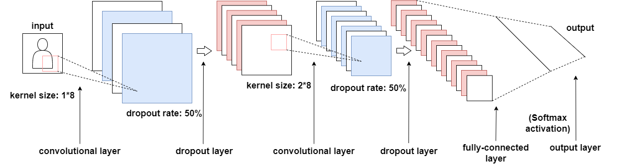
Figure 1. The convolutional neural network applied in the experiment

The deep learning model architecture processes input data with dimensions [2,1024] through a sequential structure beginning with the first convolutional layer containing 50 filters of size 1×8 with ReLU activation while maintaining the original output dimensions, followed by a dropout layer that eliminates half of the features. The data then flows into a second convolutional layer equipped with 50 filters of size 2×8, again using ReLU activation, after which another dropout layer similarly removes half of the generated features. The network subsequently incorporates a flattening layer that transforms the multidimensional data into a one-dimensional vector, which is then fully connected to 256 neurons. Before the final classification stage, a third dropout layer is applied with the same 50% dropout rate, ultimately leading to the output layer's 24 neurons that correspond to the target modulation classification categories.

3.3.2. Residual neural network

The experimental implementation utilizes a streamlined residual neural network architecture that preserves the core residual learning principles while maintaining model performance. Specific modifications were made to the input and output data processing to optimize adaptation for the automatic modulation recognition task. The complete architecture of this customized residual neural network is presented in Figure 2.

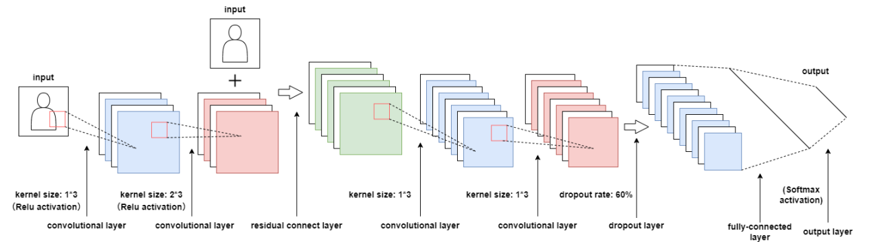
Figure 2. The residual neural network applied in the experiment

The architecture of the residual neural network, as illustrated in the figure, processes input data with dimensions [2, 1024] through the following computational pipeline. The network initially employs a residual block comprising two convolutional layers with residual connections. The first convolutional layer utilizes 256 filters of size 1×3 with ReLU activation while maintaining identical input-output dimensions, followed by a second convolutional layer with 256 filters of size 2×3, also employing ReLU activation with dimensional preservation. The residual connection enables element-wise addition between the block's input and the second convolutional layer's output, implementing the fundamental residual learning mechanism.

Subsequent to the residual block, the data flows through two additional convolutional layers, each containing 80 filters of size 1×3 with ReLU activation and dimensional consistency. Following the fourth convolutional layer, a dropout layer with a 60% dropout rate is applied for overfitting prevention. The network then transforms the processed features through a flattening layer that converts the high-dimensional data into a one-dimensional vector, which is subsequently fed into the first fully-connected layer with 128 neurons and ReLU activation, followed by another dropout layer with an identical 60% dropout rate. The final output layer consists of 24 neurons with softmax activation, generating the classification probabilities for the target modulation formats.

3.3.3. Multi-scale contextual attention network

The experimental framework employs an advanced architecture specifically optimized for processing two-dimensional input signals in automatic modulation recognition tasks. This network incorporates sophisticated hierarchical structures while preserving the essential residual connection mechanism from residual neural networks, demonstrating superior performance for modulation classification. Given the complexity of the multi-scale modules and the impracticality of exhaustive enumeration and graphical representation of all components, we provide a generalized structural description. The complete architecture of this multi-scale convolutional neural network is illustrated in the accompanying Figure 3.

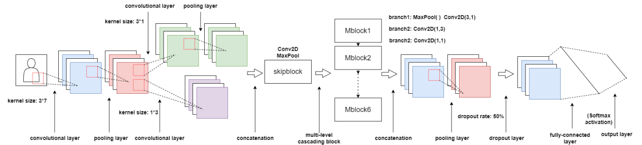
Figure 3. Multi-scale contextual attention network applied in the experiment

The network architecture processes two-dimensional input data through a carefully designed sequence of computational components, beginning with an initial convolutional block that utilizes large 3×7 kernels with double-stride implementation to efficiently capture broad spatial features while employing max-pooling for regularization. The data then flows into a dual-branch preprocessing structure where spatially separated 3×1 and 1×3 convolutional filters independently process dimensional features before hybrid pooling reduces the parameter space in preparation for the multi-branch modules.

Six distinct multi-branch modules form the core of the architecture, with the first module establishing the fundamental processing pattern: dimensionality reduction via 1×1 convolution followed by parallel processing through three separate branches applying 3×1, 1×3, and 1×1 convolutions respectively. The parallel outputs merge through concatenation before establishing residual connections with the original input, implemented through either direct addition or max-pooled addition pathways. Subsequent modules gradually increase in complexity, systematically expanding the channel depth from 32 to 96 while maintaining the triple-branch convolutional paradigm to deepen feature learning.

The final classification stage begins with global average pooling to enhance regularization before applying 50% dropout and flattening the processed features into one-dimensional representation. A fully connected layer then projects these features to the 24-dimensional output space where softmax activation generates the final classification probabilities.

This architecture demonstrates several key innovations including hybrid spatial processing through strategically sized asymmetric kernels, adaptive feature fusion via parallel processing branches, progressive channel expansion coupled with residual learning, and multi-stage regularization through combined pooling and dropout strategies. The design achieves an optimal balance between comprehensive feature extraction, computational efficiency through dimensional management, and robust performance via hierarchical representation learning.

The complete configuration is illustrated in the accompanying figure, showcasing the integrated data flow from input processing through the multi-branch feature extraction stages to final classification output. Each component contributes synergistically to the network's ability to handle complex modulation patterns while maintaining efficient computation suitable for practical implementation.

3.4. Comparison and analysis of the model performance

Following the model training under the specified experimental setup, we evaluated the performance through accuracy curves and confusion matrices. The results demonstrate that classification accuracy is highly dependent on signal-to-noise ratio (SNR) conditions, with all models exhibiting significantly better performance at higher SNR levels.

In extreme low-SNR scenarios (-20 dB and -10 dB), the models failed to distinguish between modulation schemes, consistently predicting only the most frequent modulation type in the training set. This suggests that when noise dominates the signal, the models converge to a trivial solution, losing discriminative capability.

The baseline CNN achieved 58.91% accuracy at favorable SNR levels. The ResNet architecture, incorporating residual learning, showed improved performance by better preserving temporal signal features. However, the most significant improvement came from the Multi-Branch CNN, which attained 82.39% accuracy by leveraging parallel feature extraction across multiple scales. There are also some key findings like: ResNet improved accuracy but increased training time by 50% compared to the baseline CNN. MCNet not only achieved higher accuracy but also demonstrated faster convergence, making it more suitable for practical AMR applications.

Analysis of the confusion matrices revealed some challenges in modulation-specific classification. It shows the persistent difficulties in distinguishing between PSK and QAM modulations. Higher-order QAM schemes (e.g., 64QAM vs. 256QAM) were particularly challenging at lower SNRs (<10 dB), with accuracy dropping sharply. Otherwise, reliable classification generally required SNR levels above 10 dB for most modulation types.

When it comes to the computational efficiency, while the ResNet's residual connections enhanced feature propagation, they came at a computational cost. In contrast, MCNet achieved superior efficiency by optimizing parallel processing, making it both more accurate and faster to train than the other architectures.

These results highlight the critical role of SNR in AMR performance and demonstrate that advanced architectures like the MCNet can significantly improve both accuracy and efficiency. Future work should focus on enhancing low-SNR robustness while maintaining computational efficiency for real-time applications. The detailed result of this experiment is shown in Table 2 below. The figures of the confusion matrix and the validation accuracy comparison are shown in Figures 4 to 9.

Table 2. Experiment result

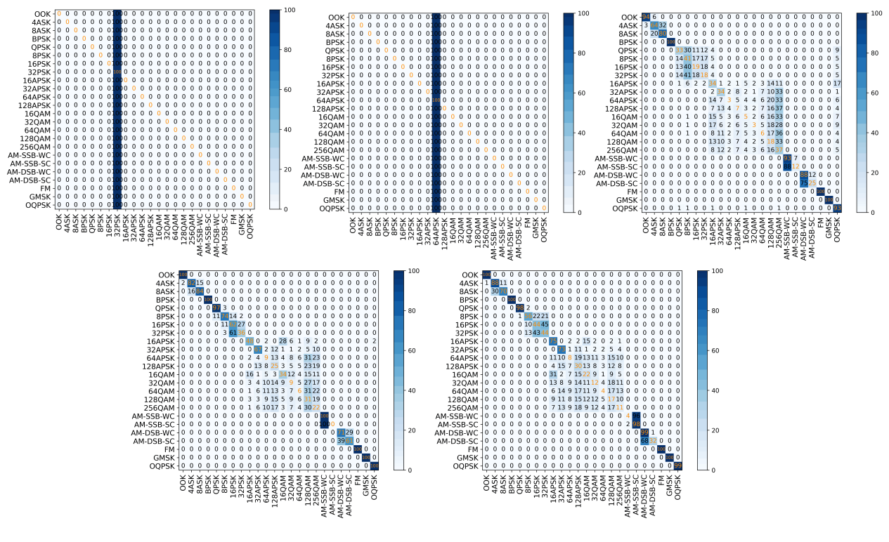
Figure 4. Confusion matrices of CNN outputs across five SNR levels

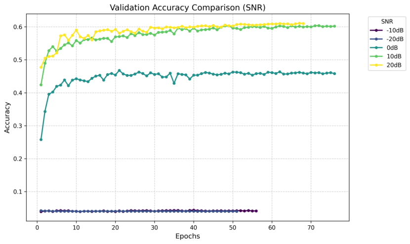
Figure 5. CNN’s validation accuracy comparison in different SNR

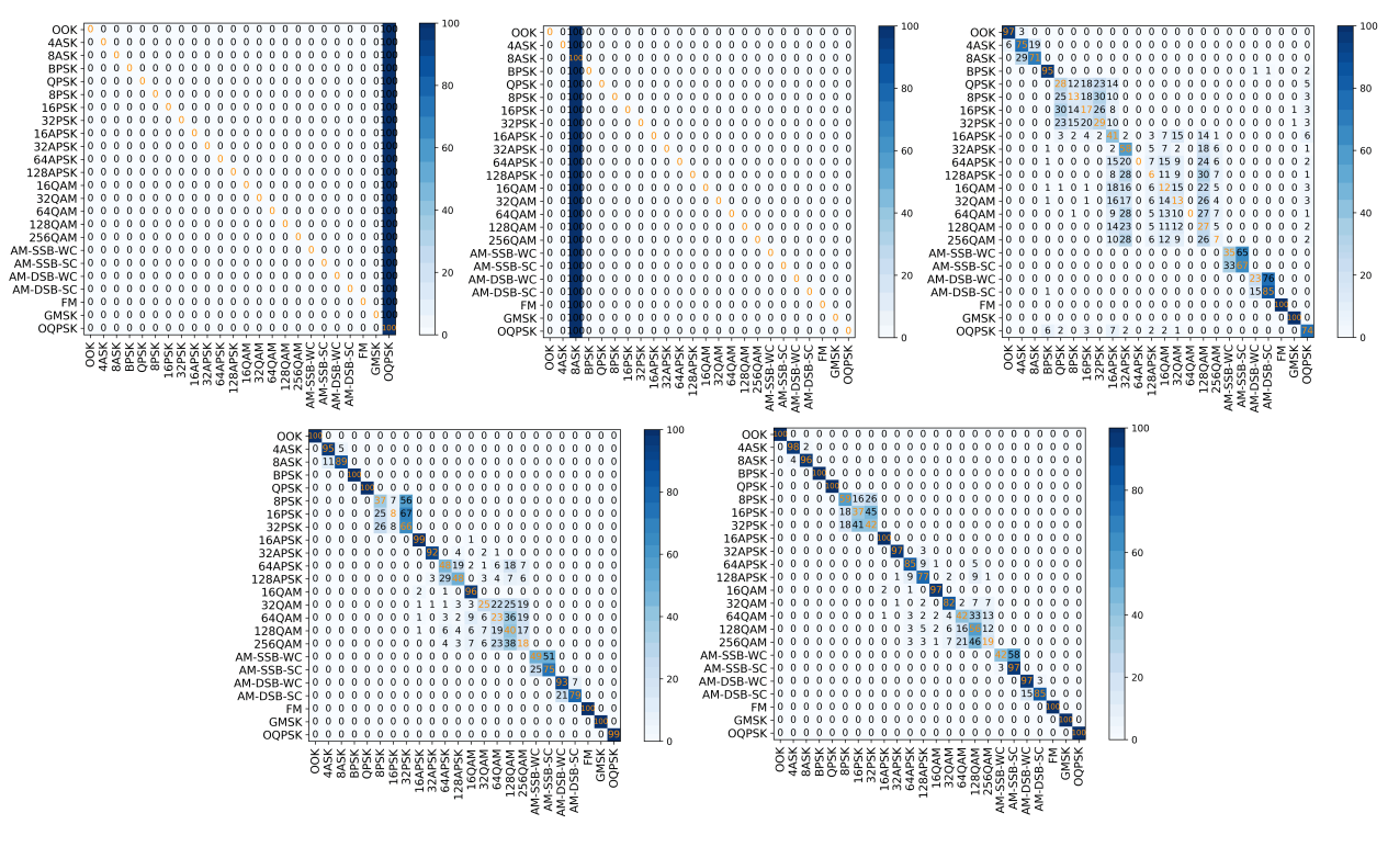
Figure 6. Confusion matrices of ResNet outputs across five SNR levels

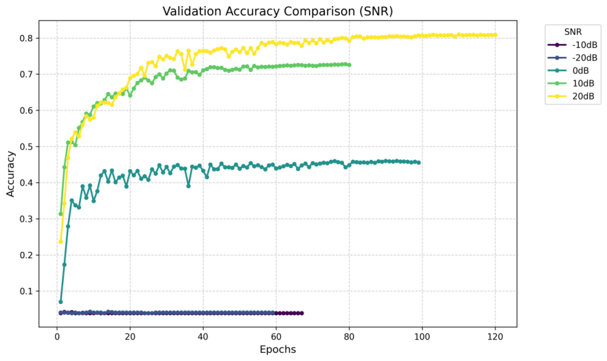
Figure 7. ResNet’s validation accuracy comparison in different SNR

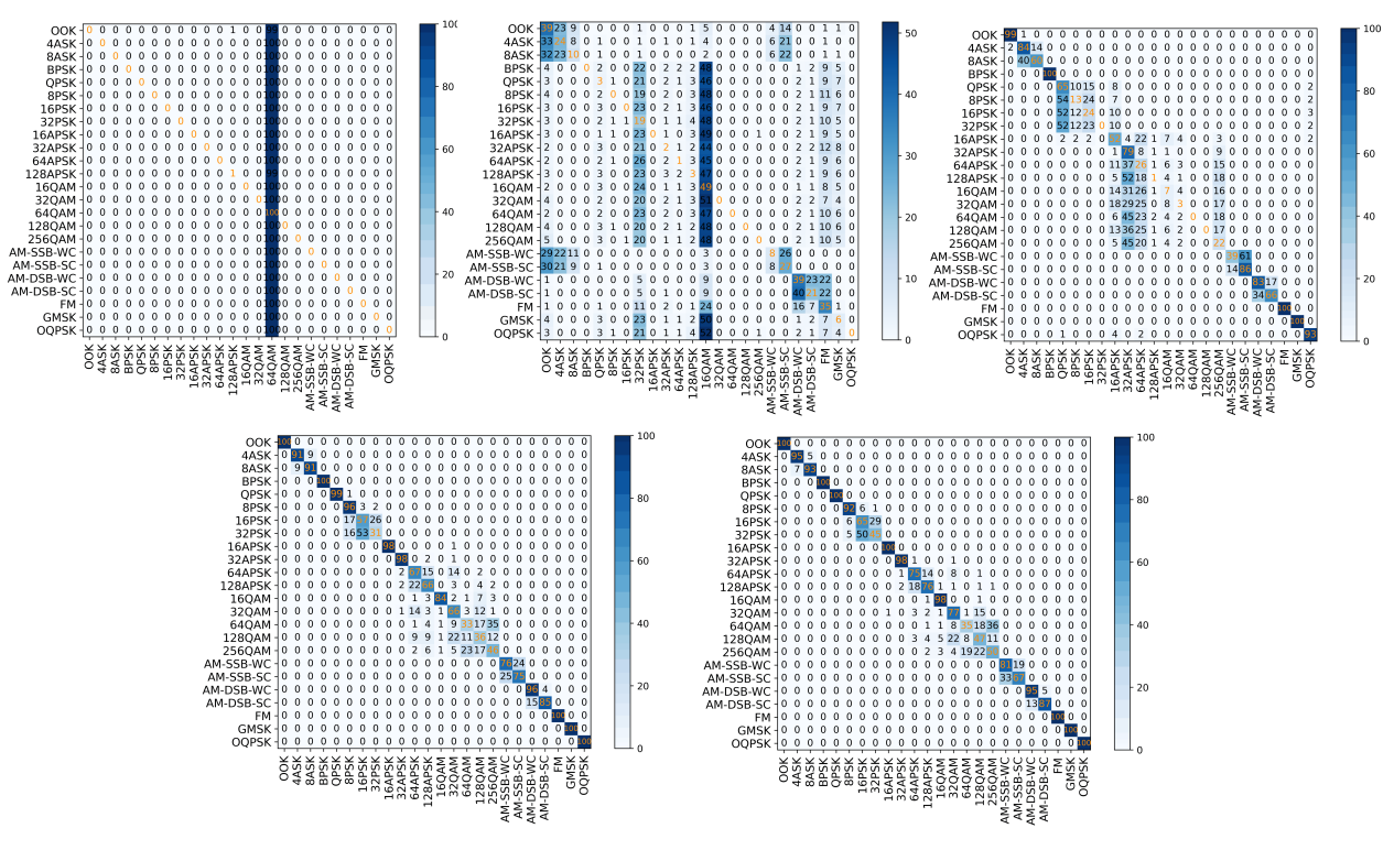
Figure 8. Confusion matrices of MCNet outputs across five SNR levels

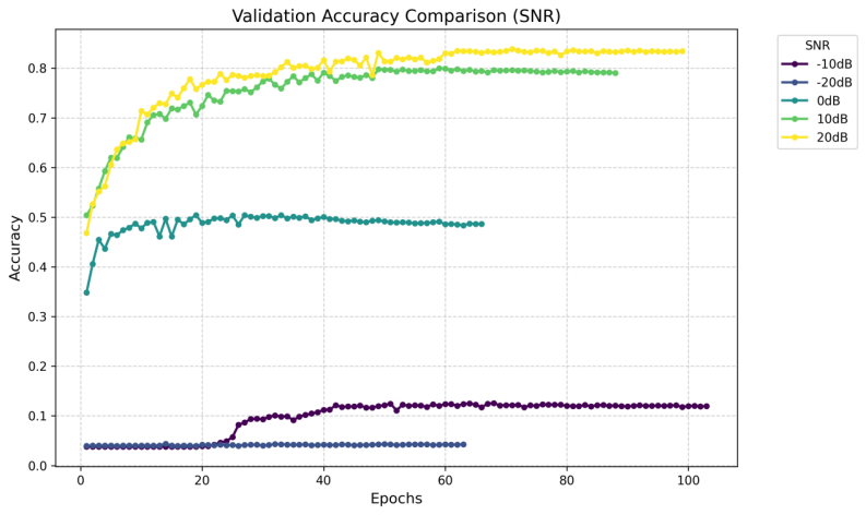
Figure 9. MCNet’s validation accuracy comparison in different SNR

4. Conclusion

This study investigates the performance of deep learning models in automatic modulation recognition (AMR), with a focus on comparative advantages and limitations across neural network architectures. Among the three selected networks, the Multi-Scale Contextual Attention Network(MCNet) demonstrated superior recognition accuracy and computational efficiency, suggesting its enhanced suitability for AMR tasks. This finding implies that the multi-scale module architecture exhibits intrinsic advantages in spectral feature extraction. While this work empirically establishes the performance hierarchy of the evaluated networks, it does not provide an in-depth theoretical analysis of how structural differences contribute to AMR adaptability. Future research should extend the current framework to develop specialized architectures for challenging modulation formats (e.g., high-order QAM/PSK). Also, it requires Investigation of hybrid approaches combining existing networks to further improve accuracy. Furthermore, fundamental studies on the relationship between network topology and RF signal feature learning are also necessary to be conducted.

References

[1]. O’Shea, T. J., Corgan, J., & Clancy, T. C. (2016). Convolutional Radio Modulation Recognition Networks. In C. Jayne & L. Iliadis (eds.), engineering applications of neural networks. EANN 2016 (Vol. 629, pp. 188-200). Springer, Cham. https://doi.org/10.1007/978-3-319-44188-7_16
[2]. Lecun, Y., Bottou, L., Bengio, Y., & Haffner, P. (1998). Gradient-based learning applied to document recognition. Proceedings of the IEEE, 86(11), 2278-2324. https://doi.org/10.1109/5.726791
[3]. Wang, N., Liu, Y., Ma, L., Yang, Y., & Wang, H. (2023). Automatic Modulation Classification Based on CNN and Multiple Kernel Maximum Mean Discrepancy. Electronics, 12(1), 66. https://doi.org/10.3390/electronics12010066
[4]. He, K., Zhang, X., Ren, S., & Sun, J. (2016). Deep Residual Learning for Image Recognition. 2016 IEEE Conference on Computer Vision and Pattern Recognition (CVPR), 770-778. https://doi.org/10.1109/CVPR.2016.90
[5]. Shafiq, M., & Gu, Z. (2022). Deep Residual Learning for Image Recognition: A Survey. Applied Sciences, 12(18), 8972. https://doi.org/10.3390/app12188972
[6]. Huynh-The, T., Hua, C.-H., Pham, Q.-V., & Kim, D.-S. (2020). MCNet: An Efficient CNN Architecture for Robust Automatic Modulation Classification. IEEE Communications Letters, 24(4), 811-815. https://doi.org/10.1109/LCOMM.2020.2968030
Cite this article
Zhang,Z. (2025). Deep learning-based Automatic Modulation Recognition: a comprehensive study. Advances in Engineering Innovation,16(5),69-77.
Data availability
The datasets used and/or analyzed during the current study will be available from the authors upon reasonable request.
Disclaimer/Publisher's Note
The statements, opinions and data contained in all publications are solely those of the individual author(s) and contributor(s) and not of EWA Publishing and/or the editor(s). EWA Publishing and/or the editor(s) disclaim responsibility for any injury to people or property resulting from any ideas, methods, instructions or products referred to in the content.
About volume
Journal:Advances in Engineering Innovation
© 2024 by the author(s). Licensee EWA Publishing, Oxford, UK. This article is an open access article distributed under the terms and
conditions of the Creative Commons Attribution (CC BY) license. Authors who
publish this series agree to the following terms:
1. Authors retain copyright and grant the series right of first publication with the work simultaneously licensed under a Creative Commons
Attribution License that allows others to share the work with an acknowledgment of the work's authorship and initial publication in this
series.
2. Authors are able to enter into separate, additional contractual arrangements for the non-exclusive distribution of the series's published
version of the work (e.g., post it to an institutional repository or publish it in a book), with an acknowledgment of its initial
publication in this series.
3. Authors are permitted and encouraged to post their work online (e.g., in institutional repositories or on their website) prior to and
during the submission process, as it can lead to productive exchanges, as well as earlier and greater citation of published work (See
Open access policy for details).