1. Introduction

In recent years, with the development of the manufacturing and tourism industries and the improvement of living standards, exploring underwater landscapes and searching for shipwrecks by submarine has become increasingly feasible. Civilian sightseeing submarines, also known as tourist submarines, are commercial manned submersibles [1-4]. Passenger volume has surged significantly in recent years, generating considerable profits and demonstrating substantial market potential and promising growth prospects. Consequently, the manufacturing of sightseeing submarines has advanced continuously. However, ensuring the safety of submarines and tourists necessitates the installation of appropriate safety equipment to prevent accidents [5-6]. It is also essential to establish comprehensive safety protocols to ensure that, even in the event of an accident, the mothership can immediately locate the cruising submarine and initiate rescue operations. Therefore, it is critical to develop effective methods for predicting the location of a missing cruising submarine to enable rapid search and rescue. Furthermore, a thorough analysis must be conducted to select appropriate rescue equipment and pre-deploy it on the mothership to facilitate timely rescue operations [7-8].

2. Establishment of the missing submarine position prediction model

Assume the mass of the cruising submarine is \( m \) , its volume is V, and the ocean current velocity is \( {v_{1}} \) . Due to variations in seawater pressure and salinity, seawater density changes with depth, thereby affecting the buoyant force acting on the submarine. However, based on literature review and calculations, the effect of salinity variation with depth on the final results in the vertical direction is negligible [9-11]. To simplify the calculations, this model only considers the influence of seawater temperature on density. When the temperature \( T \) falls within the range \( 10℃ \lt T \lt 50℃ \) , the relationship between seawater density and temperature is given by:

\( {ρ_{t}}=-3.4525×{10^{-4}}T(z)+1.029 \) (1)

where \( T(z) \) is the seawater temperature as a function of depth.

Taking the submarine's initial position as the origin, the tangent to the parallel (latitude circle) at that point is defined as the x-axis, and the tangent to the meridian (longitude line) is the y-axis. The positive direction of the x-axis points east, and the positive direction of the y-axis points south. The z-axis is perpendicular to the x–y plane and points toward the Earth's interior. The established three-dimensional Cartesian coordinate system is illustrated in Figure 1.

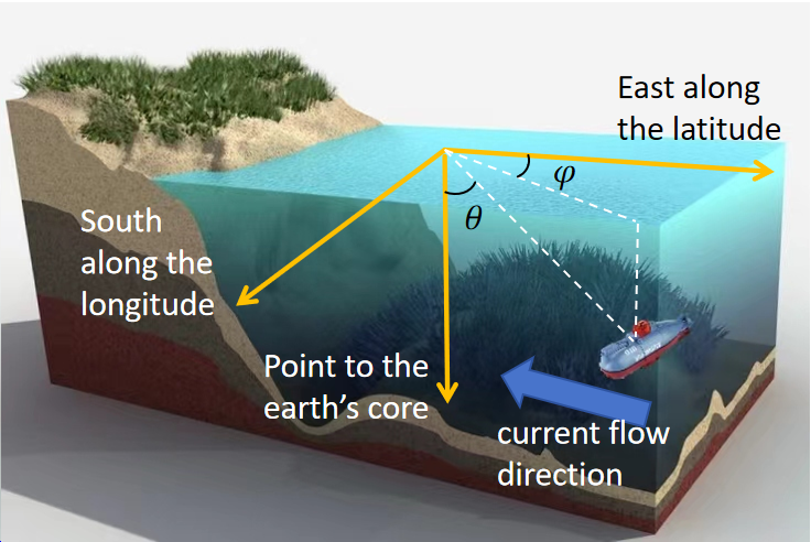
Figure 1. Schematic of the underwater cartesian coordinate system

Due to the relative motion between the submarine and the seawater, viscous drag acts on the submarine. Ignoring the irregular shape of the submarine, it is approximated as a sphere with radius \( r \) . According to Stokes' law, the viscous force acting on the submarine is:

\( {F_{η}}=-6πηr{v_{r}} \) (2)

where \( η \) is the dynamic viscosity of seawater in the region, which can be calculated by the empirical formula:

\( η=16.93×{10^{-6}}{e^{\frac{790}{{T_{p}}+273.15}}} \) (3)

where \( {T_{p}} \) is the seawater temperature. In Equation (2), \( {v_{r}} \) is the relative velocity between the submarine and the seawater, calculated as:

\( {v_{r}}={v_{0}}-{v_{1}} \) (4)

where \( {v_{0}} \) is the submarine's velocity and \( {v_{1}} \) is the ocean current velocity. The angles between the viscous force and the x-, y-, and z-axes are:

\( θ=arccos(\frac{{v_{z}}}{{v_{r}}}) φ=arcsin(\frac{{v_{x}}}{{v_{r}}sin{θ}} ) \) (5)

Moreover, due to the Earth's rotation, the submarine is subject to Coriolis force. Let the Earth's angular velocity be \( ω \) , and the submarine’s latitude be \( ψ \) . In the established coordinate system, the angular velocity vector can be expressed as:

\( ω=-ωcos{ψ}∙j+ωsin{ψ}∙k \) (6)

The Coriolis force acting on the submarine is:

\( {F_{cor}}=-2m(ω×{v_{r}}) \) (7)

Specifically:

\( \begin{cases} \begin{array}{c} {F_{xcor}}=2mω({v_{rz}}cos{ψ+}{v_{ry}}sin{ψ}) \\ {F_{ycor}}=-2mω{v_{rx}}sin{ψ} \\ {F_{zcor}}=-2mω{v_{rx}}cos{ψ} \end{array} \end{cases} \) (8)

Assuming that at the moment of mechanical failure, the submarine's buoyant force equals its gravitational force, the net forces acting on the submarine in each direction are:

\( \begin{cases} \begin{array}{c} {F_{xcor}}=2mω({v_{rz}}cos{ψ+}{v_{ry}}sin{ψ}) \\ {F_{ycor}}=-2mω{v_{rx}}sin{ψ} \\ {F_{zcor}}=-2mω{v_{rx}}cos{ψ} \end{array} \end{cases} \) (9)

From these, the accelerations and velocity changes of the submarine in each direction can be obtained:

\( \begin{cases} \begin{array}{c} \frac{d{v_{x}}}{dt}=\frac{{F_{x}}}{m} \\ \frac{d{v_{y}}}{dt}=\frac{{F_{y}}}{m} \\ \frac{d{v_{z}}}{dt}=\frac{{F_{z}}}{m} \end{array} \end{cases} \) (10)

Through the above analysis, the changes in the submarine's velocity after mechanical failure can be predicted, thereby enabling estimation of its location.

3. Preliminary prediction results

Assuming that the submarine is located at a point in the Mediterranean Sea (18°E, 37°N) and is descending vertically with an initial velocity of \( {v_{z}}=0.5m/s \) , the submarine's motion trajectory under different loss-of-power depths can be predicted, as shown in Figure 2.

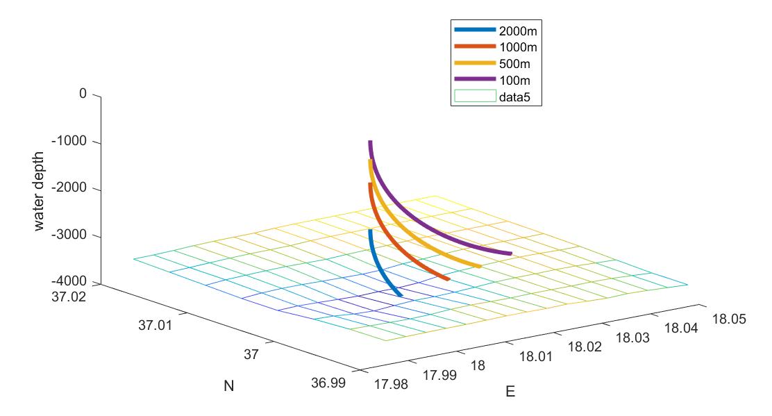
Figure 2. Preliminary trajectory prediction

It can be observed that, due to the influence of the Coriolis force, the submarine’s descent trajectory is not a straight line but a spiral. The final landing points are summarized in Table 1.

Table 1. Final landing points

4. Uncertainties in the model

Clearly, real-world ocean conditions are more complex than those considered in the simplified model, particularly regarding ocean currents [12-13]. The flow velocity of seawater varies with depth. Surface currents are primarily influenced by trade winds and thermodynamic factors [14], while deep-sea currents are affected by seabed topography, tides, and other factors. Based on research data, the vertical profile of seawater flow velocities at the study location (18°E, 37°N) is shown in Figure 3.

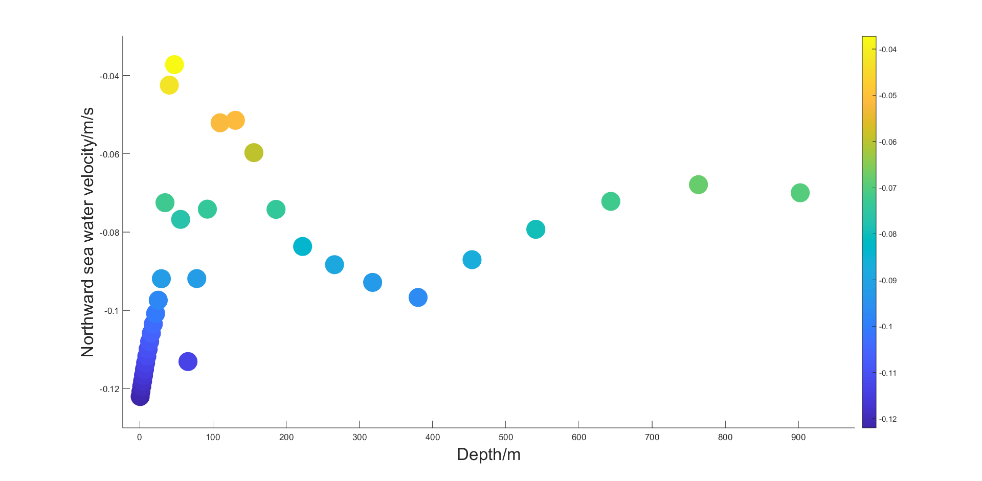
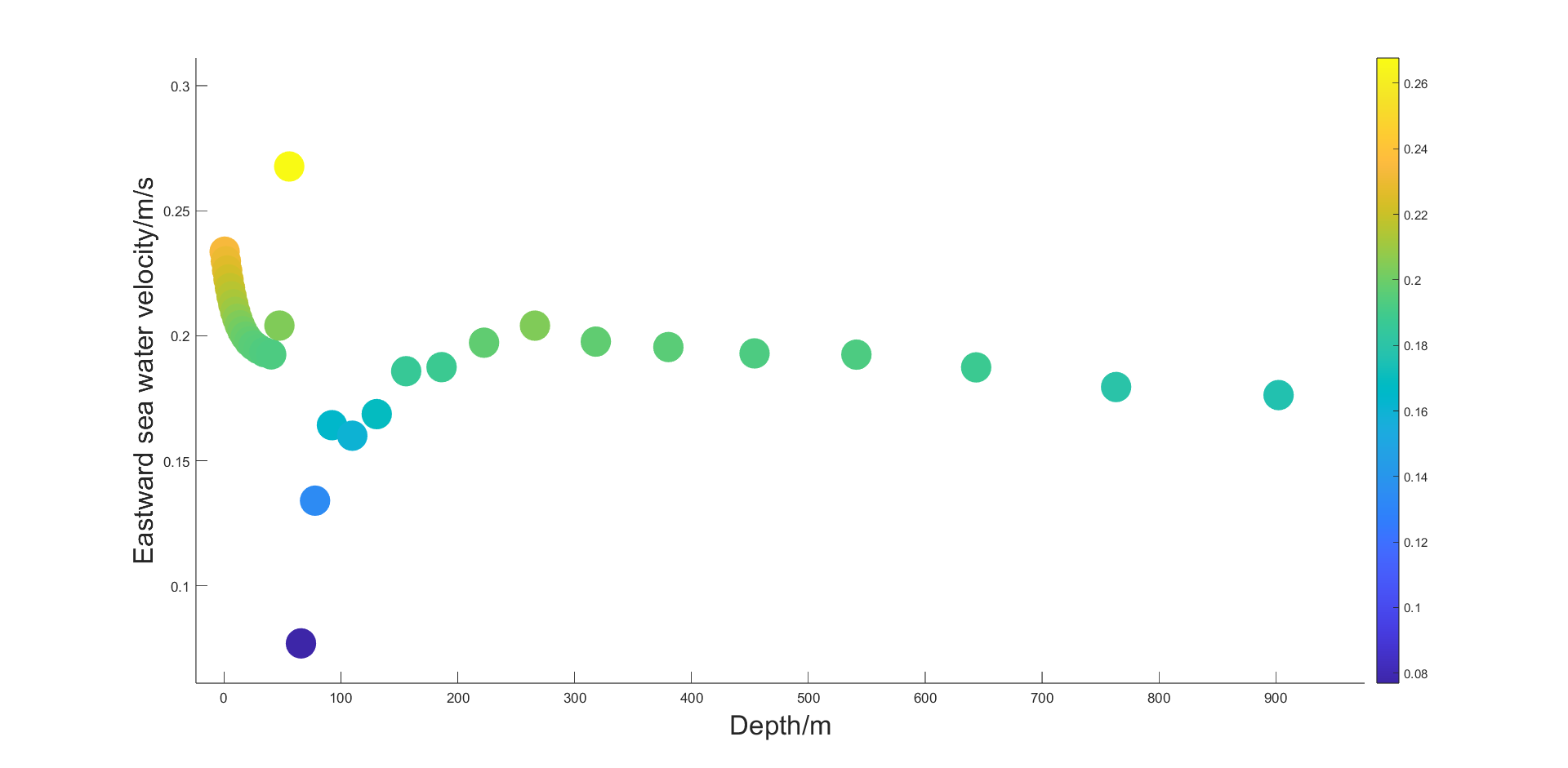
Figure 3. (a) Northward seawater flow velocity (b) Eastward seawater flow velocity

After incorporating the varying seawater flow velocities at different depths into the model, the predicted trajectory of the submarine post-power-loss is updated as shown in Figure 4.

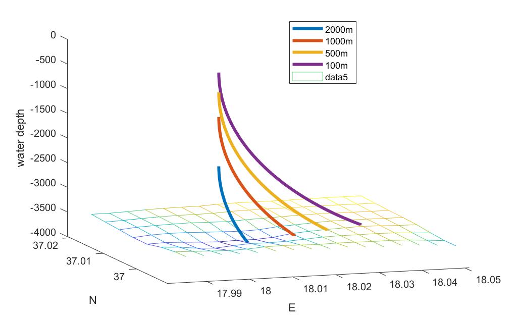
Figure 4. Trajectory prediction considering real ocean currents

The final landing points under these more realistic conditions are given in Table 2.

Table 2. Final landing points under realistic ocean current conditions

It can be seen that the actual offset of the submarine differs from the predictions based on uniform seawater conditions, especially when the submarine loses power at shallower depths. At shallow depths, the variability in current speed is more significant, resulting in larger discrepancies in final landing points. In contrast, at greater depths, where ocean current velocities vary less, the prediction error is relatively smaller. Thus, equipping submarines with seawater flowmeters is critically important for rescue operations.

Additionally, the submarine's trajectory is influenced by several factors, including the depth at which it loses power, its initial descent velocity, and the location of the incident.

Figure 5 illustrates the trajectories under different initial velocities ( \( 0.1m/s \) , \( 0.4m/s \) , \( 0.7m/s \) ) at a loss-of-power depth of 100 meters at 18°E, 37°N.

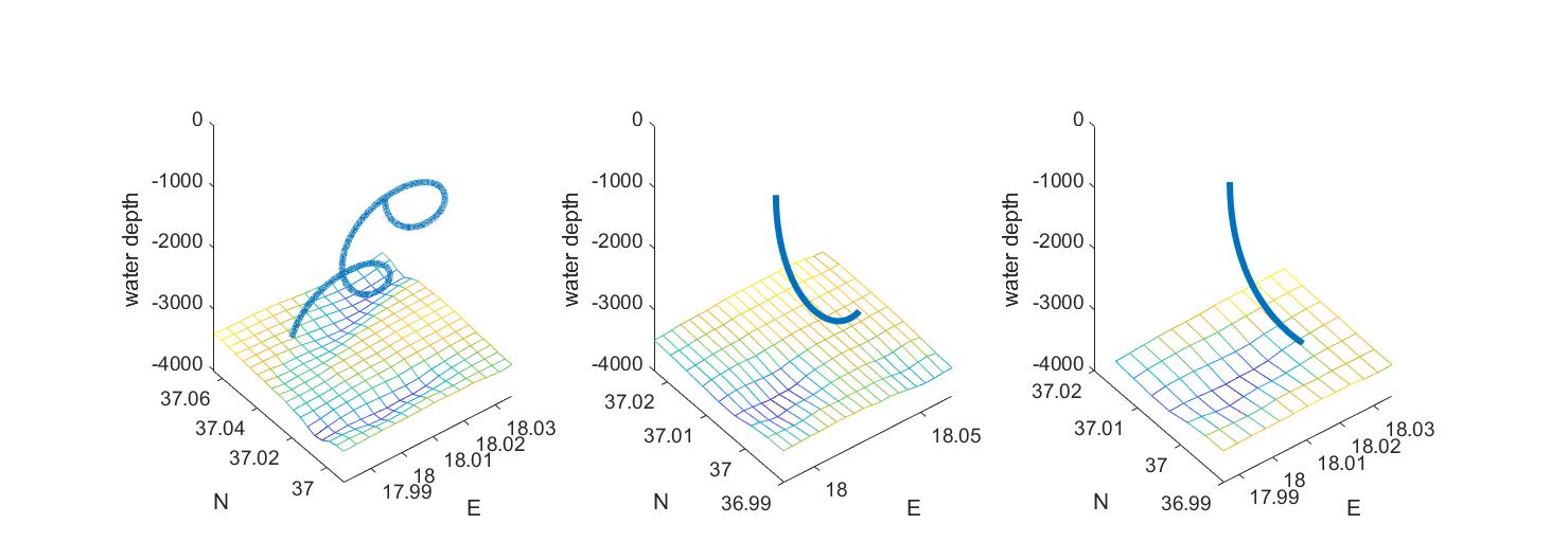
(a) (b) (c)

Figure 5. Submarine trajectories at different initial velocities(a) \( {v_{z}}=0.1m/s \) (b) \( {v_{z}}=0.4m/s \) (c) \( {v_{z}}=0.7m/s \)

When the initial descent velocity is 0.4 m/s and the power loss occurs at 100 meters depth, the effect of different incident locations on the trajectory is shown in Figure 6.

(a) (b) (c)

Figure 6. Submarine trajectories at different incident locations(a) \( 36.6°N 17.6°E \) (b) \( 37.2°N 18.2°E \) (c) \( 37.8°N 18.8°E \)

It can be observed that a slower initial descent velocity leads to a longer time to reach the seabed and a greater horizontal offset from the original position. Moreover, during the later stages of descent, the radius of the spiral motion caused by the Coriolis force increases, further amplifying the positional uncertainty.

The depth at which the submarine loses contact primarily affects the time required to reach the seabed—the deeper the loss-of-contact point, the quicker the submarine reaches the seabed, though rescue operations become more challenging due to the increased distance from the surface.

Furthermore, varying incident locations alter seafloor topography and local current patterns, influencing the descent trajectory. Biological activities, density variations in seawater, and other factors can also affect the submarine's path, significantly increasing the complexity and difficulty of rescue operations [15].

5. Ensuring safety

Based on the above analysis, to enable timely rescue operations following a submarine’s loss of contact, it is critical that the cruising submarine regularly transmits its status to the mothership. Key information should include: Position (coordinates and depth). Submarine’s physical characteristics (mass, volume). Operational status (velocity, local seawater current speed) By leveraging this real-time data, the mothership can predict the submarine’s future trajectory, narrow the search area, and greatly enhance the chances of successful rescue operations.

References

[1]. Chen, B., Li, R., Bai, W. J., Li, J. X., & Guo, R. (2019). Multi-DOF Motion Simulation of Underwater Robot for Submarine Cable Detection. In B. Xu (Ed.) IEEE 8th Joint International Information Technology and Artificial Intelligence Conference (ITAIC).
[2]. Chen, Y. R., Liang, S. Q., Yang, G. Q., Wang, L., Zhou, Y. G., & Tian, X. Q. (2023). A New Method for Locating Positions of Single-Core Cables in Three-Phase Submarine Power Circuits Based on Phase Difference Data. Ieee Access, 11, 107906-107916. http://doi.org/10.1109/ACCESS.2023.3321094
[3]. Cheng, X. Z., Shu, H. N., Liang, Q. L., & Du, D. (2008). Silent positioning in underwater acoustic sensor networks. Ieee Transactions On Vehicular Technology, 57(3), 1756-1766.
[4]. Duan, C. F., Kuang, C. L., Zhang, H. N., Sang, K. W., Yang, B. C., & Ruan, F. M. (2024). Multisensor Fusion Positioning for Marine Towed Streamers: Modeling, Evaluation, and Comparison. Ieee Transactions On Instrumentation and Measurement, 73 http://doi.org/10.1109/TIM.2024.3418091
[5]. Gao, R. R., Xu, T. H., Ai, Q. S., & IEEE. (2017). Research on Underwater Sound Velocity Calculation, Error Correction and Positioning Algorithms 2017 FORUM ON COOPERATIVE POSITIONING AND SERVICE (CPGPS) (39-42). Forum on Cooperative Positioning and Service (CPGPS).
[6]. Li, G., Feng, H., Huang, M., & Xu, H. (2009). Study and simulation of the positioning model of Underwater multi-streamer. Technical Acoustics, 28(2), 113-116.
[7]. Li, X. S., Li, W. B., Mao, Z. Y., & Zhang, Y. (2017). Multiple Anti-submarine Helicopters' Cooperative Front Submarine Detecting Research. In H. Zhou & Z. Xu (Eds.), 5th International Conference on Frontiers of Manufacturing Science and Measuring Technology (FMSMT).
[8]. Liu, Y. T., Wu, Y. Q., Li, G., Abbas, A., & Shi, T. K. (2024). Submarine cable detection using an end-to-end neural network-based magnetic data inversion. Journal of Geophysics and Engineering, 21(3), 884-896.
[9]. Song, Y., Ye, H. J., Wang, Y. H., Niu, W. D., Wan, X., & Ma, W. (2021). Energy Consumption Modeling for Underwater Gliders Considering Ocean Currents and Seawater Density Variation. Journal of Marine Science and Engineering, 9(11) http://doi.org/10.3390/jmse9111164
[10]. Liu, Q., Liu, D., Bai, J., Zhang, Y. P., Zhou, Y. D., Xu, P. T., Liu, Z. P., Chen, S., Che, H. C., Wu, L., Shen, Y. B., & Liu, C. (2018). Relationship between the effective attenuation coefficient of spaceborne lidar signal and the IOPs of seawater. Optics Express, 26(23), 30278-30291. http://doi.org/10.1364/OE.26.030278
[11]. Tenzer, R., Novák, P., & Gladkikh, V. (2011). On the accuracy of the bathymetry-generated gravitational field quantities for a depth-dependent seawater density distribution.
[12]. Miao, Y. J., Dong, X. L., Bourassa, M. A., Du, Y., Zhu, D., & IEEE. (2022). THE DEMAND OF TOTAL OCEAN SURFACE CURRENT MEASUREMENT IEEE International Geoscience and Remote Sensing Symposium (IGARSS).
[13]. Dohan, K. (2017). Ocean surface currents from satellite data. Journal of Geophysical Research-Oceans, 122(4), 2647-2651. http://doi.org/10.1002/2017JC012961
[14]. Zhou, P. Z., Jiao, K. K., Wang, Z. H., Cheng, X., Zhang, X. D., & IEEE. (2022). An ocean current prediction method for profiling float based on RBFNN 2022 OCEANS HAMPTON ROADS. OCEANS Hampton Roads Conference.
[15]. Zhou, L., Zhao, Q. S., Chi, S. K., Liu, L. J., Yu, Q. X., & IEEE. (2017). Research on Underwater Device Positioning Method in Deep Water Controllable Source Electromagnetic Exploration System 2017 IEEE INTERNATIONAL CONFERENCE ON SIGNAL PROCESSING, COMMUNICATIONS AND COMPUTING (ICSPCC). IEEE International Conference on Signal Processing, Communications and Computing (ICSPCC).
Cite this article
Zhang,J. (2025). A dynamic model-based approach for predicting the position of a missing submarine. Advances in Engineering Innovation,16(5),63-68.
Data availability
The datasets used and/or analyzed during the current study will be available from the authors upon reasonable request.
Disclaimer/Publisher's Note
The statements, opinions and data contained in all publications are solely those of the individual author(s) and contributor(s) and not of EWA Publishing and/or the editor(s). EWA Publishing and/or the editor(s) disclaim responsibility for any injury to people or property resulting from any ideas, methods, instructions or products referred to in the content.
About volume
Journal:Advances in Engineering Innovation
© 2024 by the author(s). Licensee EWA Publishing, Oxford, UK. This article is an open access article distributed under the terms and
conditions of the Creative Commons Attribution (CC BY) license. Authors who
publish this series agree to the following terms:
1. Authors retain copyright and grant the series right of first publication with the work simultaneously licensed under a Creative Commons
Attribution License that allows others to share the work with an acknowledgment of the work's authorship and initial publication in this
series.
2. Authors are able to enter into separate, additional contractual arrangements for the non-exclusive distribution of the series's published
version of the work (e.g., post it to an institutional repository or publish it in a book), with an acknowledgment of its initial
publication in this series.
3. Authors are permitted and encouraged to post their work online (e.g., in institutional repositories or on their website) prior to and
during the submission process, as it can lead to productive exchanges, as well as earlier and greater citation of published work (See
Open access policy for details).