1. Introduction

In geometry, a boundary refers to the set of points whose neighborhoods contain non-object points, without occupying any spatial extent. In images, a contour refers to the set of pixels within a target object whose 4- or 8-neighborhoods (assuming square pixels) contain object pixels; unlike points, pixels occupy space [1,2]. Contours are one of the fundamental features in images, representing the basic shape of objects and storing important information about the boundary and the entity itself (such as perimeter and area). Therefore, contour tracing is a fundamental task in image processing and computer vision, and the accuracy and reliability of its results directly affect the understanding of the real world [3,4]. The earliest known contour tracing techniques can be traced back to the 1960s [5], proposed by researchers such as Robert L. K. Tukey and Paul Viola. Although this research has a history of over 60 years, the number of available techniques remains small, and their evolution has been very slow. For example, the widely used and important findContours function in OpenCV relies on the 1990s radical sweep method and topological analysis based on Suzuki’s 1985 method [6, 7].

Traditional contour tracing algorithms can be broadly categorized into three types: pixel-based tracing algorithms, vertex-based tracing algorithms (proposed in 1982) [8], and run data-based tracing algorithms (proposed in 1997 [9] and improved in 1999 [10]). Vertex-based algorithms require storing and tracking vertices instead of pixels, increasing storage requirements by at least four times and consuming significant memory while offering similar iterative performance. Run data following still has unresolved issues at 8-connected junctions and requires further refinement. Additionally, these methods are complex to implement and integrate. Vertical run data tracing involves frequent allocation and deallocation of pointers, and direct scanning must consider background pixels, leading to low efficiency for complex boundaries. As a result, their development has stagnated. Pixel-based tracing algorithms, thanks to Suzuki’s method, are better at analyzing topological structures and easier to implement, making them more widely used and the main focus of researchers. Nevertheless, traditional techniques have several critical limitations.

First, they cannot capture all contour pixels. Their strategy of simultaneously searching for and identifying contour pixels leads to missed pixels due to search limitations. Methods like MNT and RSA fail to trace inner corner pixels and achieve only about 82% accuracy [11]. Even the more accurate ISBF and FCTA methods achieve close to 99.5% but still fall short of 100%. The proposed technique first identifies all contour pixels (while extracting enclosed object information, which previous methods could not achieve) and then classifies these pixels using run data (e.g., distinguishing inner and outer boundaries). Based on the definition of contour pixels and a predefined scanning strategy, this approach can locate 100% of all contour pixels.

Second, highly accurate traditional methods are slow and memory-intensive because they trace contours one at a time. To avoid misidentifying non-start pixels as start points, they must complete one tracing before starting the next, disrupting the scanning process and introducing costly small loops. They also require recording starting points and entry directions, consuming significant memory. Overlapping paths result in repeated pixel tracing, wasting computational resources. Algorithms like FCTA further increase computational load by evaluating pixel region patterns at each step. In contrast, the proposed method scans the entire image from top-left to bottom-right without being interrupted by individual tracing processes, ensuring high computational speed. It avoids frequent entry into individual tracing routines, eliminating the need to record starting points and entry directions, thus saving memory. By capturing all contour pixels first and performing classification later, it improves computational efficiency.

Third, traditional methods cannot provide detailed, diverse representations of contour topology. Because they fail to capture all contour pixels, they cannot represent topological structures in detail. They only supply contour pixels without additional information, limiting their representational capacity and preventing them from determining which entity a given contour belongs to. The proposed technique increases the information content of contour pixels by adding new features and expanding pixel vectors, enabling more diverse and detailed representations of contour topology.

Since 2016, the fundamental nature of contour tracing algorithms has not changed [12-14]. Most researchers have focused on parallelizing existing methods [12] or integrating them with neural networks. However, these approaches have not fundamentally solved the problem: accuracy remains limited, and speed continues to encounter bottlenecks.

To address these issues, this paper proposes a new run data algorithm, further parallelized using MPI to improve its speed.

The paper consists of three parts: the first defines basic concepts; the second describes the proposed contour tracing algorithm in detail and its application to contour topology representation; and the third validates the algorithm’s performance, efficiency, and practicality.

2. Principles of the serial novel run data algorithm

First, using the region labeling algorithm, the image is scanned for the first time to identify all boundary pixels, assign initial labels to each pixel, and record the cluster (connected region) associated with each sub-pixel area.

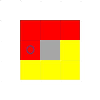
For each pixel, its upper neighborhood is scanned (using an 8-neighborhood mode with a default scan from the top-left to the bottom-right), as shown in Figure 1.

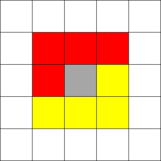
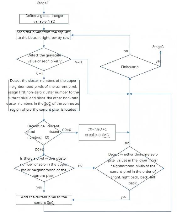
Relative to the current pixel, its upper neighborhood (the red region) has already been scanned and consists either of background pixels or entity pixels that have already been labeled. If any entity pixel exists in the red region, the label of the first such pixel encountered is assigned to the current pixel. If a background pixel is detected during the scan, the current pixel is marked as a boundary pixel. If all pixels in the upper 4-neighborhood are background pixels, a new label is created and assigned to the current pixel, and this label is added to the global label variable. If two or more different labels are found in the upper 4-neighborhood, all of these labels in the label set are unified to the smallest of them. A flowchart of this process is shown in Figure 2.

The following example, shown in Figure 3, illustrates this process.

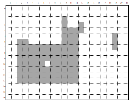
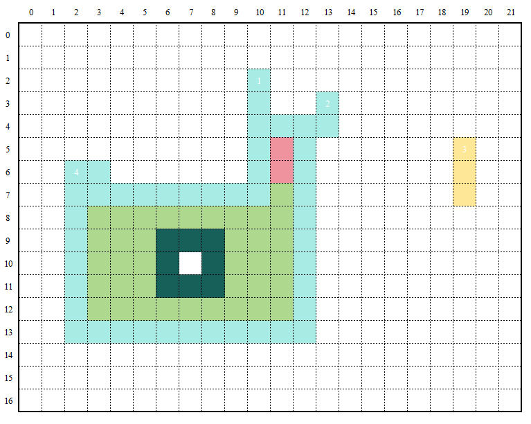
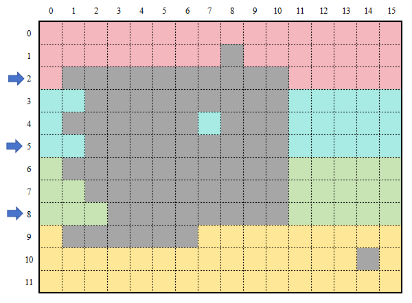
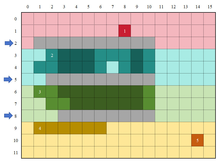
After Stage 1, all boundaries are extracted, and the image is segmented into four parts as shown in Figure 4.

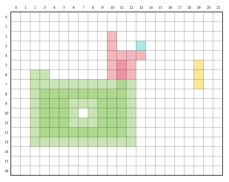
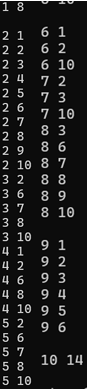
At this point, the global set of labels is obtained:

$$ label\mathrm{ }=\mathrm{ }\left\{1,\mathrm{ }1,\mathrm{ }3,\mathrm{ }1\right\}$$(1)

The purpose of maintaining this label set is to enable merging of subregions that belong to the same connected area. For example, regions 1, 2, and 4 are actually connected and should be treated as a single region, but they were initially divided into three subregions, so labeling is necessary for subsequent merging.

In the figure, the light-colored areas represent the boundaries of regions with the same color (using the 4-neighborhood as an example). Here, the green region's boundary is divided into two parts: one part directly contacts the background (the outer contour), while the other part is caused by a white hole in the middle (the inner contour). In some applications [4], distinguishing these is unnecessary, but in others [3], such as identifying minerals surrounding rocks, it is essential to differentiate between inner and outer boundaries. Therefore, the next tasks are to merge pixels (especially boundary pixels) that belong to the same connected region and to distinguish between inner and outer boundaries based on user requirements.

At this stage, depending on user needs—such as calculating the area—synchronous statistics can also be performed.

Stage2: Using the label vector obtained in Stage 1, this step merges the boundaries of connected sub-pixel regions. During this process, the algorithm only merges information and boundaries—for example, summing areas, accumulating surrounding mineral content, or removing unwanted components—thus ensuring functionality while reducing computational load.

Step1:

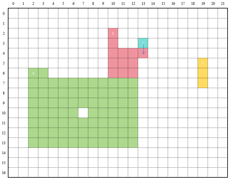
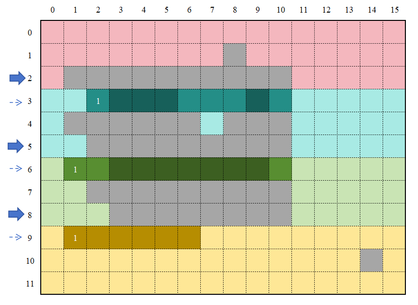
Merge regions 1 and 2 (see Figure 5).

$$ label\mathrm{ }=\mathrm{ }\left\{1,\mathrm{ }1,\mathrm{ }3,\mathrm{ }1\right\}$$(2)

Step2:

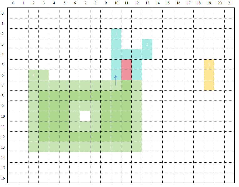
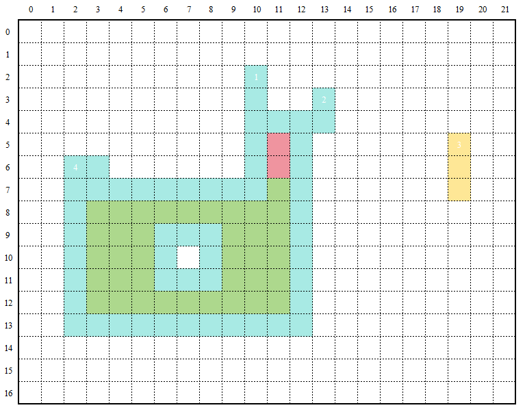
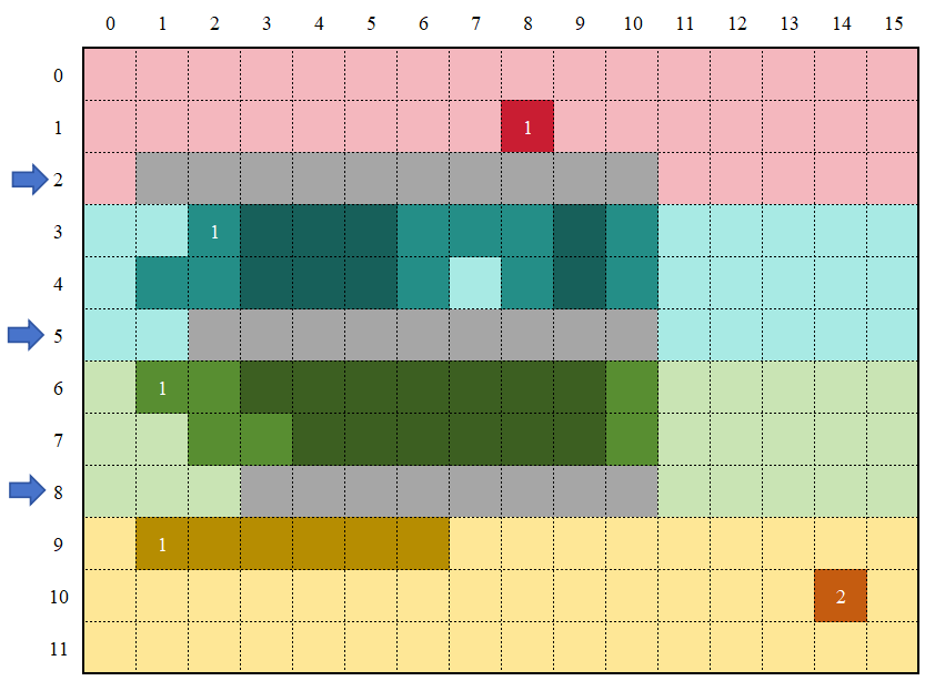
Merge regions 1 and 3 (see Figure 6 and 7).

$$ label\mathrm{ }=\mathrm{ }\left\{1,\mathrm{ }1,\mathrm{ }3,\mathrm{ }1\right\}\to \left\{1,\mathrm{ }1,\mathrm{ }3,\mathrm{ }1\right\}$$(3)

$$ label\mathrm{ }=\left\{1,\mathrm{ }1,\mathrm{ }3,\mathrm{ }1\right\}$$(4)

A summary of the process in Step 2 is provided in the flowchart shown in Figure 8.

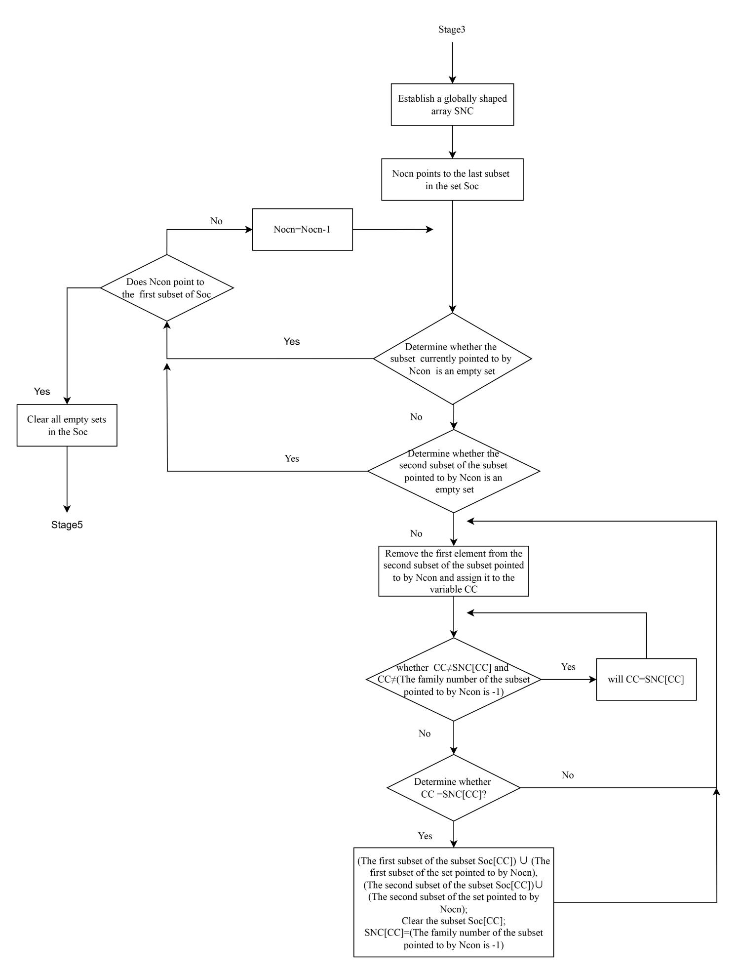
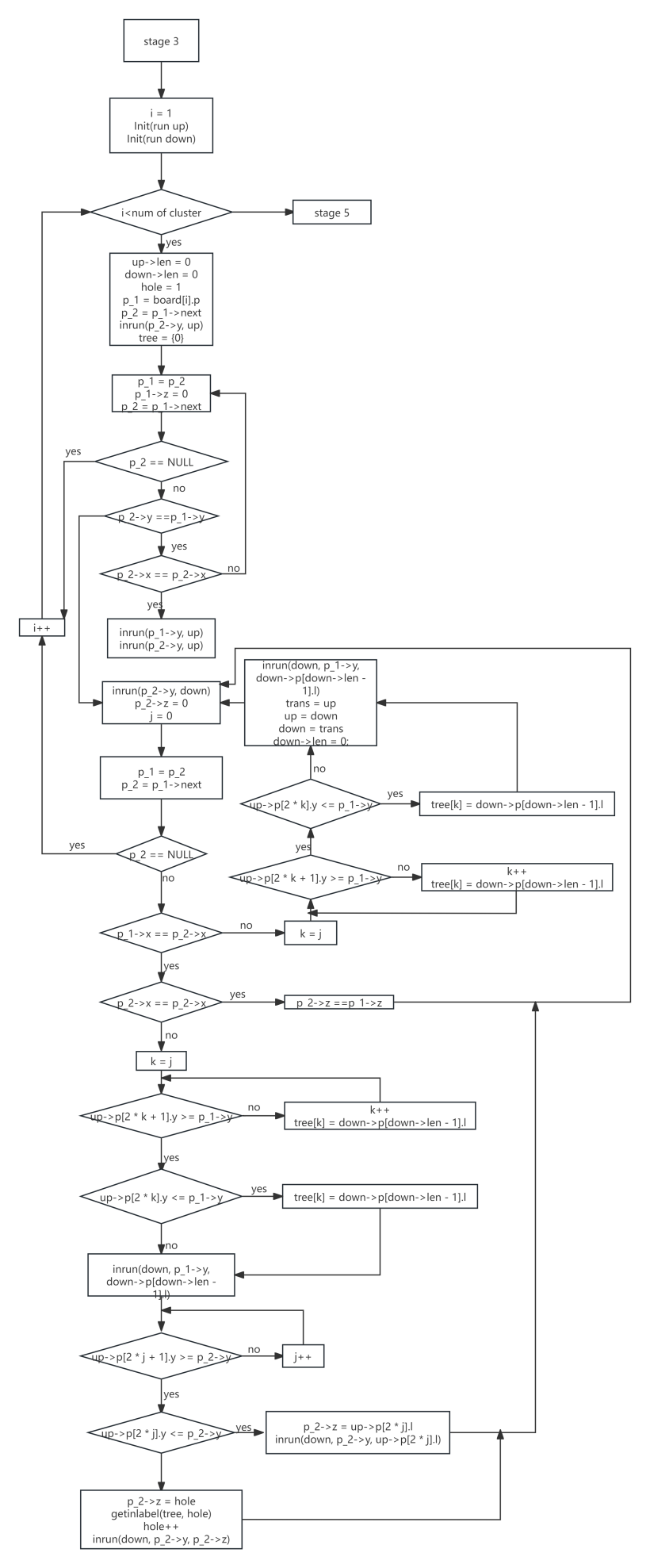
Stage3: For each connected region boundary, this step distinguishes between outer and inner contours. By integrating the run data approach [10], the algorithm determines the boundary type of the current scan line using the boundary types from the previous line, following the decision process shown in the flowchart. This enables differentiation between inner and outer boundaries, as well as between multiple distinct inner boundaries.

The flowchart for this process is shown in Figure 9.

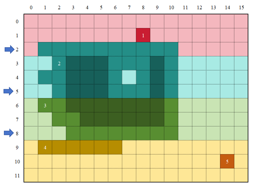
Through these stages, all boundaries are successfully extracted. The result is shown in Figure 10,

where the darker regions indicate inner boundaries.

3. Experiments with the serial algorithm

The following presents the results obtained using programs implemented in C++ and Python.

Experiment 1: C++ implementation on a specific example.

Original image (Figure 11, from the MPEG7-CE standard dataset)

The processing time for each stage is shown in Table 1:

It can be observed that Stage 1 consumes the most time. Subsequent parallelization efforts will focus on this module.

The tracked boundaries are shown in Figure 12:

A magnified detail is shown in Figure 13:

Here, dark blue indicates outer boundaries, while light blue indicates inner boundaries. In this example, the large butterfly shape contains many holes not belonging to the main butterfly, resulting in situations where light blue regions are nested within dark blue regions.

Experiment 2: Comparison with traditional algorithms.

The comparison was conducted under the following hardware and software configuration (see Table 2):

The comparison is made against OpenCV (known as cv2 in Python). The results include tests with the latest official release as well as the 2024 first-half-year version (see Table 3):

In terms of accuracy, the widely used OpenCV implementation achieves less than 80%, a figure also supported by [11] (82%). The latest boundary-tracing algorithm [11] claims to achieve 97% accuracy, which holds for simple images; however, our experiments show that for complex images, it reaches only around 90%. In contrast, our method completely extracts all boundaries without removing or introducing any spurious boundaries during processing, thus achieving 100% accuracy (as shown in the last column).

The following figure shows a time comparison between our algorithm and OpenCV (see Figure 14):

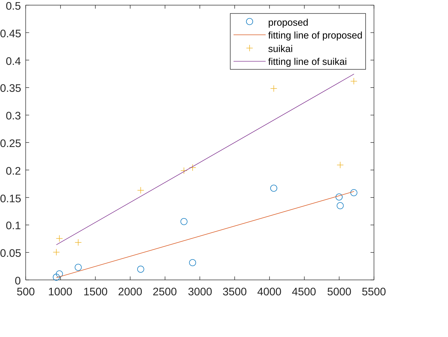
(x-axis represents the number of boundary pixels; y-axis represents time in seconds)

Compared to traditional algorithms, the proposed method offers 100% accuracy along with higher processing speed.

4. A new MPI-based parallel run data algorithm

From the above comparison of processing times across different stages, it is clear that Stage 1 is the most time-consuming. Therefore, parallelization will first be applied to Stage 1. The primary reason for Stage 1’s high computational cost lies in the fact that, in the serial implementation, pixel scanning is performed by a single processor [12,15]. Inspired by the multiprocessor system approach of parallel boundary-tracing algorithms [12], this method introduces multiple processors during the scanning process to improve speed.

Unlike traditional tracing processes, here each processor is assigned both an initial scanning point and a specific scanning region. Thus, the entire image is divided into multiple scanning regions, with the number of regions determined by the number of CPU cores and the image size. After each processor completes scanning its designated region, specialized processing is performed on boundary pixels at region interfaces (since their upper four neighbors may not have been fully scanned yet). Additionally, the labels of subregions are reassigned and merged as necessary.

The first step is image partitioning. To simplify boundary handling and ensure balanced computational workload, the image is evenly divided along rows, as shown in Figure 15 and 16.

Different colors indicate different scanning regions. The division is performed by rows, so the same object may be split across multiple regions. In the example above, the object is divided into four parts. Three boundary pixel runs are highlighted with arrows [10].

Next, special handling is required for the row immediately following a division line (the “second divided row”), because pixels in this row do not have all four upper neighbors labeled, making normal serial-style scanning impossible.

Therefore, the scanning process for pixels in the second divided row is modified as shown in Figure 17:

For these pixels, only the left neighbor has been scanned. Therefore, the algorithm uses the original labeling strategy for the left neighbor (determining boundary status and assigning labels), while for other neighbors it simply checks their values without modifying the cluster label.

The resulting labeling is shown in Figure 18, where solid arrows indicate division lines and dashed arrows indicate the second divided rows:

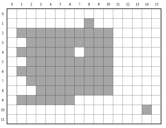
For all other rows within each region (excluding the division and second divided rows), scanning proceeds in the same manner as in the serial implementation. The result after scanning in this example is shown in Figure 19:

In the figure, the darker colored regions represent the identified interior pixels of the object, while the lighter colored regions (still darker than the background) represent the boundary pixels of the corresponding region. After scanning, the results from different regions are merged and the labels are reassigned, as shown in Figure 20:

Finally, specialized scanning is applied to the boundary pixel runs, as illustrated in Figure 21:

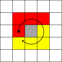
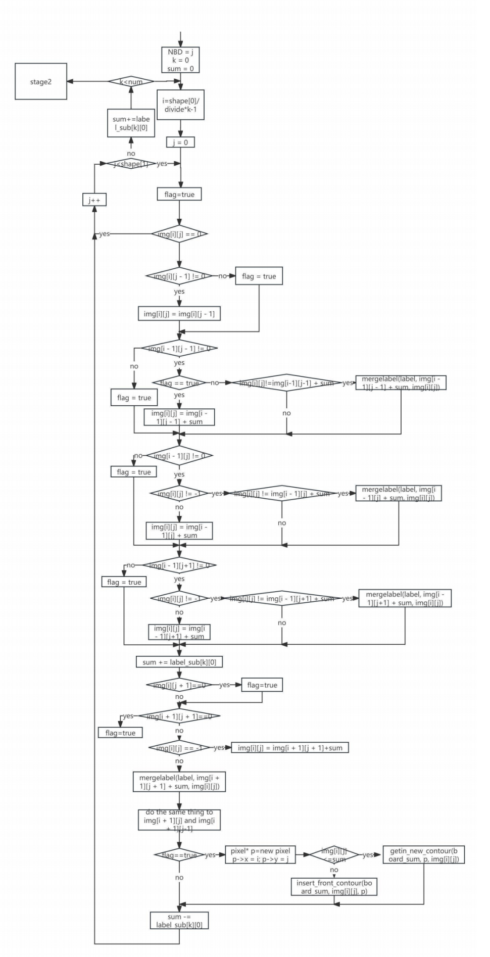
In the serial implementation, for both boundary and non-boundary pixels, scanning proceeds clockwise: first the upper four neighbors, then the lower four. This is because the upper neighbors have already been scanned, so starting with them ensures correct labeling. However, in the parallel case, for boundary pixels, not only are the upper four neighbors scanned, but all lower neighbors except the left neighbor have also been processed. Therefore, the scanning order is modified as shown in Figure 22:

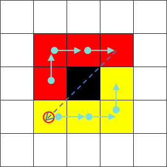
Specifically, after scanning the upper four neighbors, the algorithm proceeds counterclockwise starting from the lower-left neighbor. For the example above, the resulting labeling is shown in Figure 23:

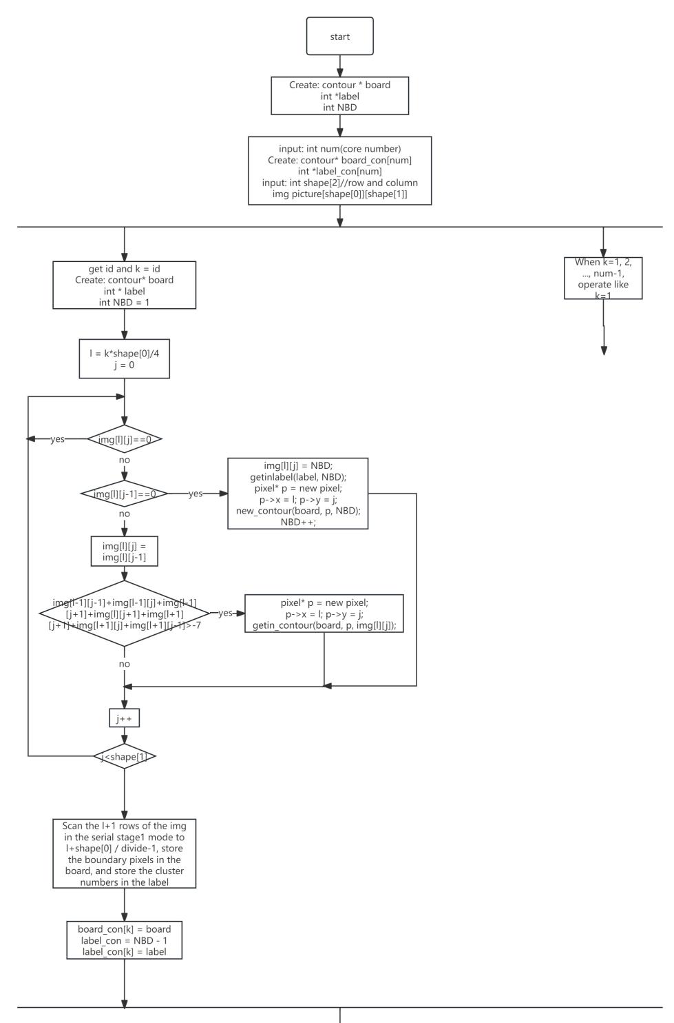
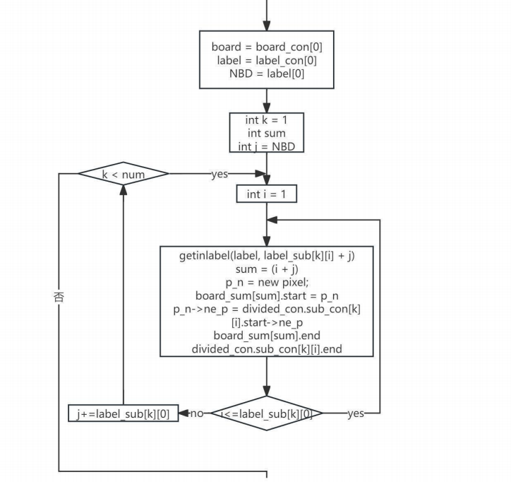
The above algorithm design translates into three main programming steps: first, parallel scanning of the original image; second, merging and relabeling of the boundary and region sets after aggregation; and finally, special handling for the division lines.

The overall workflow is summarized in Figure 24-26:

5. Parallel algorithm experiments

The following experiments are divided into two parts: first, verifying the accuracy of this approach, and second, comparing its speed.

Experiment 1: Parallel Contour Extraction on a Specific Example

The original image is shown in Figure 27:

The image properties are shown in Figure 28:

The extracted contour pixels are shown in Figure 29:

From the results, it is evident that the extracted boundaries match the true contour pixels exactly—neither more nor less.

Experiment 2: The experimental environment is summarized in Table 4, and the results comparing the parallel and serial algorithms are given in Table 5.

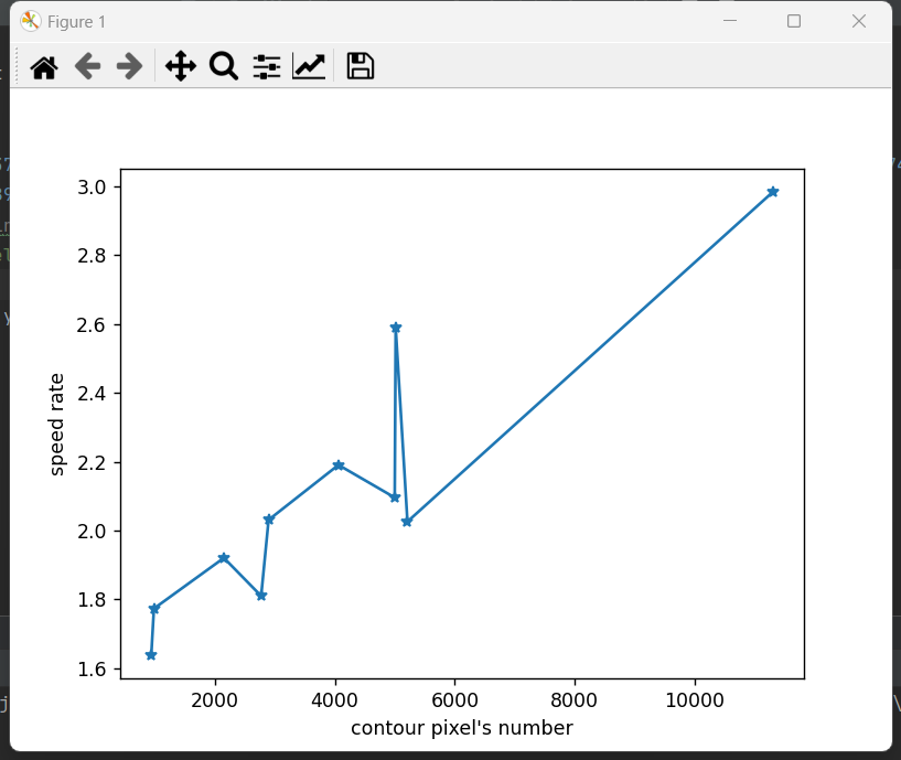
From the results in Figure 30, it can be seen that the parallel algorithm is faster than the serial algorithm. Moreover, the speedup increases as the number of boundary pixels grows. Its theoretical upper limit is 4, as approximated by the formulas (5) and (6) given in [15].

$$ W=W_s+W_p$$(5)

$$ S=\frac{W}{W_S+W_P/P}$$(6)

6. Conclusion

To achieve 100% extraction of object boundary pixels and to establish a direct link between boundaries and their corresponding objects, this paper proposes a new boundary-tracing algorithm by combining traditional boundary-tracing methods with connected-component labeling techniques. Experiments conducted on the MPEG7-CE standard dataset demonstrate that the proposed method achieves a 100% extraction rate, producing a set of boundary pixels directly associated with the objects. Moreover, compared with existing methods of similar functionality, it achieves a significant speed improvement (at least 15%). In addition, this paper introduces an MPI-based parallel implementation of the proposed algorithm. Compared to the serial version, the parallel implementation consistently achieves speedups of at least 1.64× and up to 2.98×. This further improves efficiency, making the method more suitable for accurate large-scale image boundary extraction and tracing. Future work will explore modeling the containment relationships between different objects and their boundaries, as well as extending the boundary-tracing approach to three-dimensional or even n-dimensional images.

Funding project

National Natural Science Foundation of China (42374152); Shandong Provincial Natural Science Foundation (ZR2020MD050)

References

[1]. Cheong, C. H., & Han, T. D. (2006). Improved simple boundary following algorithm.Journal of KIISE: Software and Applications,33(4), 427-439.
[2]. Hu, J., Kang, J., Zhang, Q., Liu, P., & Zhu, M. (2018). An improved eight-neighborhood image boundary tracking algorithm.Bulletin of Surveying and Mapping,(12), 21-25.
[3]. Bolelli, F., Allegretti, S., & Grana, C. (2022). Connected Components Labeling on Bitonal Images. InInternational Conference on Image Analysis and Processing(pp. 347-357). Cham: Springer International Publishing.
[4]. Liu, X., Wang, J., Ge, L., Hu, F., Li, C., Li, X., ... & Xue, Q. (2017). Pore-scale characterization of tight sandstone in Yanchang Formation Ordos Basin China using micro-CT and SEM imaging from nm-to cm-scale.Fuel,209, 254-264.
[5]. Rosenfeld, A. (1970). Connectivity in digital pictures.Journal of the ACM (JACM), 17(1), 146-160.
[6]. Suzuki, S. (1985). Topological structural analysis of digitized binary images by border following.Computer vision, graphics, and image processing,30(1), 32-46.
[7]. Li, H. (2024). A target contour tracking method based on Siamese network.Computer Engineering and Science,46(12), 2215–2226.
[8]. Li, Z., Yokoi, S., Toriwaki, J., & Fukumura, T. (1982).Border following and reconstruction of binary pictures using grid point representation.Trans. Inst. Electron. Commun. Eng. Japan [Part D] J,65, 1203-1210.
[9]. Miyatake, T., Matsushima, H., & Ejiri, M. (1997). Contour representation of binary images using run-type direction codes.Machine Vision and Applications,9, 193-200.
[10]. Shoji, K., Miyamichi, J., & Hirano, K. (1999). Contour following and reconstruction of binary images stored in run format.Systems and Computers in Japan,30(11), 1-11.
[11]. Seo, J., Chae, S., Shim, J., Kim, D., Cheong, C., & Han, T. D. (2016). Fast contour-tracing algorithm based on a pixel-following method for image sensors.Sensors,16(3), 353.
[12]. Gupta, S., & Kar, S. (2022). Algorithms to speed up contour tracing in real time image processing systems.IEEE Access, 10, 127365-127376.
[13]. Saye, R. I. (2022). A connected component labeling algorithm for implicitly-defined domains. arXiv preprint arXiv: 2205.14885.
[14]. Bhattacharya, P. (1996). Connected component labeling for binary images on a reconfigurable mesh architecture.Journal of systems architecture,42(4), 309-313.
[15]. Chen, H. (2018).High-performance parallel computing. China University of Petroleum Press.
Cite this article
Xiao,J.;Jiu,J. (2025). A new contour tracing algorithm based on run data and its parallel design and implementation. Advances in Engineering Innovation,16(7),1-20.
Data availability
The datasets used and/or analyzed during the current study will be available from the authors upon reasonable request.
Disclaimer/Publisher's Note
The statements, opinions and data contained in all publications are solely those of the individual author(s) and contributor(s) and not of EWA Publishing and/or the editor(s). EWA Publishing and/or the editor(s) disclaim responsibility for any injury to people or property resulting from any ideas, methods, instructions or products referred to in the content.
About volume
Journal:Advances in Engineering Innovation
© 2024 by the author(s). Licensee EWA Publishing, Oxford, UK. This article is an open access article distributed under the terms and
conditions of the Creative Commons Attribution (CC BY) license. Authors who
publish this series agree to the following terms:
1. Authors retain copyright and grant the series right of first publication with the work simultaneously licensed under a Creative Commons
Attribution License that allows others to share the work with an acknowledgment of the work's authorship and initial publication in this
series.
2. Authors are able to enter into separate, additional contractual arrangements for the non-exclusive distribution of the series's published
version of the work (e.g., post it to an institutional repository or publish it in a book), with an acknowledgment of its initial
publication in this series.
3. Authors are permitted and encouraged to post their work online (e.g., in institutional repositories or on their website) prior to and
during the submission process, as it can lead to productive exchanges, as well as earlier and greater citation of published work (See
Open access policy for details).