1. Introduction

Accurate stock price forecasting remains a pivotal challenge in financial analytics, primarily due to the dual complexity of modelling linear trends and nonlinear volatility inherent in market data. Traditional statistical models, while effective for stationary series, struggle with abrupt market shifts, whereas machine learning approaches demand substantial computational resources. While traditional methods like the ARIMA model excel at modeling linear relationships, they fall short when dealing with complex nonlinear patterns. Although deep learning models such as LSTM can capture nonlinear features, they have relatively high requirements for computing resources and data scale. In recent years, the ARIMA-LSTM hybrid model has emerged as a new direction for improving prediction accuracy by combining the strengths of linear and nonlinear modeling. In this paper, we use the stock price data of Apple Inc. (AAPL) from 2016 to 2024 as the research object. The prediction performance of ARIMA, LSTM, and ARIMA-LSTM hybrid models is systematically compared, and a hybrid modeling framework based on residual remapping is proposed. The key contributions of this paper are as follows:

1. Verifying the efficient performance of the hybrid model in stock price forecasting.

2. Demonstrating the internal mechanism of synergistic optimization of linear and nonlinear components.

3. Proposing a dynamic feature fusion method for dealing with extreme events.

Based on the empirical results, the predictive performance of the model in stock price forecasting is comprehensively validated, and a fundamental analysis of its mechanisms is systematically conducted. Finally, practical recommendations for model implementation and potential directions for future research are thoroughly discussed

2. Literature review

Early research results proposed the ARIMA model [1], which models stationary sequences through differencing and autoregressive moving average terms. However, the model’s neglect of nonlinear features limits its application to complex financial data. The LSTM network proposed by [2] solves the gradient vanishing problem of RNN through a gating mechanism and has become an important tool for time series prediction. In recent years, hybrid models (e.g., ARIMA-LSTM) have shown potential in fields such as power load forecasting [3], exchange rate forecasting [4], and financial time series analysis [5, 6]. The results show that by decomposing the linear and nonlinear components, the hybrid model can significantly improve the prediction accuracy [7]. Nevertheless, the application of these hybrid models in stock price forecasting still needs to be verified and explored. Building on these foundations, our analysis extends hybrid modeling to equity price forecasting, with a focus on addressing extreme market conditions.

3. Data source and preprocessing

Source: Daily adjusted closing prices of Apple Inc. (AAPL) from April 1, 2016, to January 3, 2024 (data source: Yahoo Finance).

Preprocessing Steps:

4. Missing Value Processing: Linear interpolation is used to fill in the missing data (missing rate < 0.1%).

5. Outlier Correction: Extreme values are eliminated based on the 3σ principle (data for 3 trading days in total).

6. Normalization: Min-Max normalization is applied to scale the data to the [0, 1] interval.

Dataset Division: Training Set: April 1, 2016 – December 31, 2021. (Data from 2022 was excluded from both training and testing sets to alleviate market anomalies after the pandemic)

Test Set: January 1, 2023 – January 3, 2024 (this period is chosen to avoid interference from the abnormal data that occurred during COVID-19).

4. Model construction and principles

4.1. ARIMA model

Principal Overview:

ARIMA (Autoregressive Integrated Moving Average Model) is based on the following three components to model the linear relationships in a time series:

1. Autoregressive (AR): Assumes a linear relationship between the current value and past values.

2. Differencing (I): Transforms a non-stationary sequence into a stationary sequence through differencing operations.

3. Moving Average (MA): Assumes a linear relationship between the current value and past error terms. By differencing non-stationary time series to make them stationary, the model can then use the AR and MA components to capture the autocorrelation and randomness of the series, enabling the prediction of future values.

Parameter determination:

1. The sequence is stationary after the first-order difference is confirmed by ADF test (d=1);

2. ACF is truncated at the second order of hysteresis (q=2), PACF is truncated at the first order of hysteresis (p=1), and the final model is ARIMA (1,1,2).

4.2. LSTM model

principal Overview:

LSTM (Long Short-Term Memory) is a special type of Recurrent Neural Network (RNN) that introduces gating mechanisms (forgetting gates, input gates, output gates)

1. Input Gate: Controls the extent to which new information enters the memory unit.

2. Forget Gate: Decide what information in the memory unit needs to be forgotten.

3. Output Gate: Determines what information needs to be output in the memory unit.

Selectively memorize and forget information to solve the gradient vanishing problem of traditional RNNs, so that long-term dependencies in long series data can be effectively handled.

Parameter determination:

1. Input layer: time step = 10 (price for the last 10 days);

2. Hidden layer: 2 layers of LSTM, 128 neurons per layer (activation function = Tanh);

3. Output Layer: Fully Connected Layer (Activation Function = Linear).

4. Learning rate = 0.001, batch size = 32, iterations = 100, Dropout = 0.2.

5. Actual prediction performance and analysis of ARIMA model and LSTM model

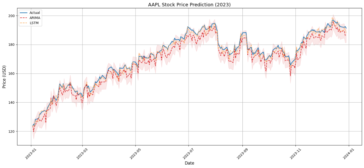
Figure 1. ARIMA vs. LSTM prediction performance (2023-2024)

5.1. ARIMA model performance

• The stationary linear trend part performed better: As shown in figure 1, from mid-September 2023 to early October 2023, the price change was relatively stable, and the forecast value of the ARIMA model (red dotted line) was close to the actual value (blue solid line), which means that the ARIMA model has a good prediction effect on this linear trend.

• Limited predictive power during high volatility: As shown in figure 1, in early September 2023 and early November 2023, prices fluctuated greatly, and the ARIMA model's forecasts deviated significantly from actual values, making it impossible to effectively predict these sharp fluctuations.

5.2. LSTM model performance

• Better at capturing complex non-linear fluctuations: As shown in figure 1, in early September 2023 and early November 2023, the LSTM model's forecasts (orange dotted line) were closer to the actual values and were better able to predict these sharp fluctuations.

• The range in which the forecast value is closer to the actual value: As shown in figure 1, from mid-November 2023 to mid-December 2023, the forecast value of the LSTM model is in good agreement with the actual value, which means that the LSTM model has a better ability to fit the nonlinear price fluctuations at this stage.

5.3. Conclusion

In summary, the ARIMA model performs well in the smooth linear trend part but has limited prediction ability in the case of severe fluctuations. The LSTM model performs better at capturing complex nonlinear fluctuations, especially when prices change dramatically, and the predicted values are closer to the actual values than the ARIMA model

6. Construction idea of ARIMA-LSTM hybrid model

The essence of the ARIMA-LSTM hybrid model is the residual remapping mechanism, which is divided into three steps: [8]

1. The ARIMA model deals with the linear part [9]:

• Use ARIMA models to model time series data and capture linear trends.

• The ARIMA model can effectively process stationary or differentially processed non-stationary data through differential, autoregressive and moving average operations.

2. The LSTM model deals with the non-linear part [10]:

• The residuals of the ARIMA model were used as the input of the LSTM model, and the gating mechanism of the LSTM was used to capture the nonlinear features in the residuals.

• LSTMs are capable of handling long-term dependencies in time series, especially for complex nonlinear patterns.

3. Fusion of prediction results [11]:

• Add the predicted value of ARIMA and the predicted value of LSTM to obtain the final prediction result.

• The weighted average method can also be used to dynamically adjust the weights of the two to further optimize the prediction effect.

Figure 2. ARIMA-LSTM hybrid model architecture

Figure 2 shows that, through the above processing, it is theoretically analyzed that the ARIMA-LSTM hybrid model will show better adaptability when dealing with data with obvious linear trends or complex nonlinear data.

7. Actual prediction performance and analysis of ARIMA-LSTM model

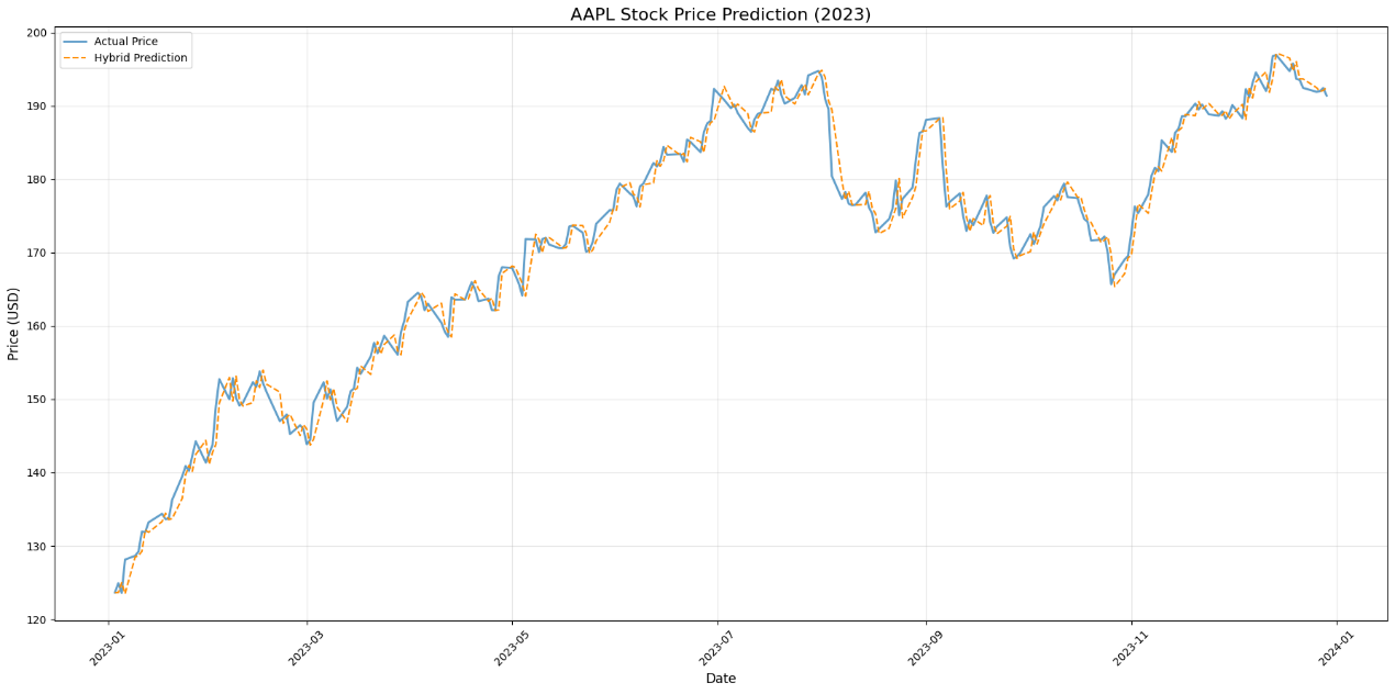
Figure 3. Hybrid model prediction vs. actual prices

This chart shows the actual value of the AAPL stock price (solid blue line) and the forecast value of the ARIMA-LSTM hybrid model (orange dotted line):

1. Overall performance

As shown in figure 3, the predicted value (orange dotted line) of the hybrid model is relatively close to the actual value overall, indicating that the hybrid model can predict the overall trend of the price well.

2. Performance during periods of extreme volatility

As shown in figure 3, around October 2023, the price fluctuates greatly, and the prediction value of the hybrid model can also predict the change of the actual value relatively well in these volatile regions, indicating that it has a good effect when dealing with nonlinear fluctuation data.

3. Stability of the model

As shown in figure 3, at the beginning of 2023, the price showed a relatively stable trend, and the forecast value of the hybrid model basically coincided with the actual value, indicating that the performance of the model during the stable period was very stable. During the period from July 2023 to October 2023, the price rose rapidly, and the prediction value of the hybrid model can also follow this trend well, indicating that the model has a good prediction effect on both stable and rapid changes in prices.

4. Error analysis

As shown in figure 3, during the period from October 2023 to December 2023, the price fluctuated greatly, and there were some deviations between the forecast and the actual value, which may be due to some unexpected factors in the market or the company.

In summary, the ARIMA-LSTM hybrid model performs well in dealing with AAPL stock price predictions and can better capture the price trend in both volatile and stable periods. This model combines the advantages of linear and nonlinear modelling and can adapt to a variety of time series data to provide more accurate predictions.

8. Comparison of the effects and deconstruction of the advantages of the three models

Next, we used the three models to determine the value of Skewness, Kurtosis, JB test p-value, RMSE (root mean square error), MAE (mean absolute error), R² (coefficient of determination), training time (seconds), and direction accuracy. The performance of these eight aspects is shown in the figure 4 and figure 5, simultaneously, the comparison and the advantages are analysed [12].

8.1. Comparison and advantage analysis of model performance (skewness, kurtosis, JB test p-value)

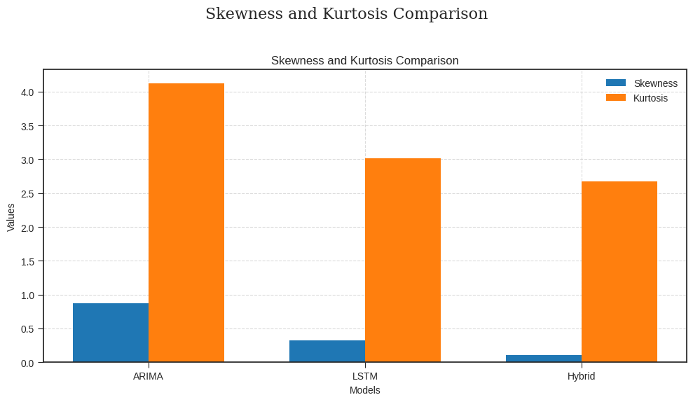
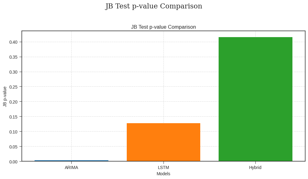
Figure 4. Statistical distribution comparison (skewness & kurtosis)

• Skewness: ARIMA (0.87, right bias, asymmetric data processing limitations) > LSTM (0.32, close to symmetry) > hybrid model (0.11, optimal symmetry).

• Kurtosis: ARIMA (4.12, insufficient robustness of thick tail distribution) > LSTM (3.01, near-normal) > hybrid model (2.67, best normal fit).

• JB test p-value: ARIMA (0.003, significantly deviating from normal) < LSTM (0.127) < hybrid model (0.415, error distribution closest to normal).

8.2. Comparison and advantage analysis of statistical characteristics (RMSE, MAE, R²), training time and direction accuracy

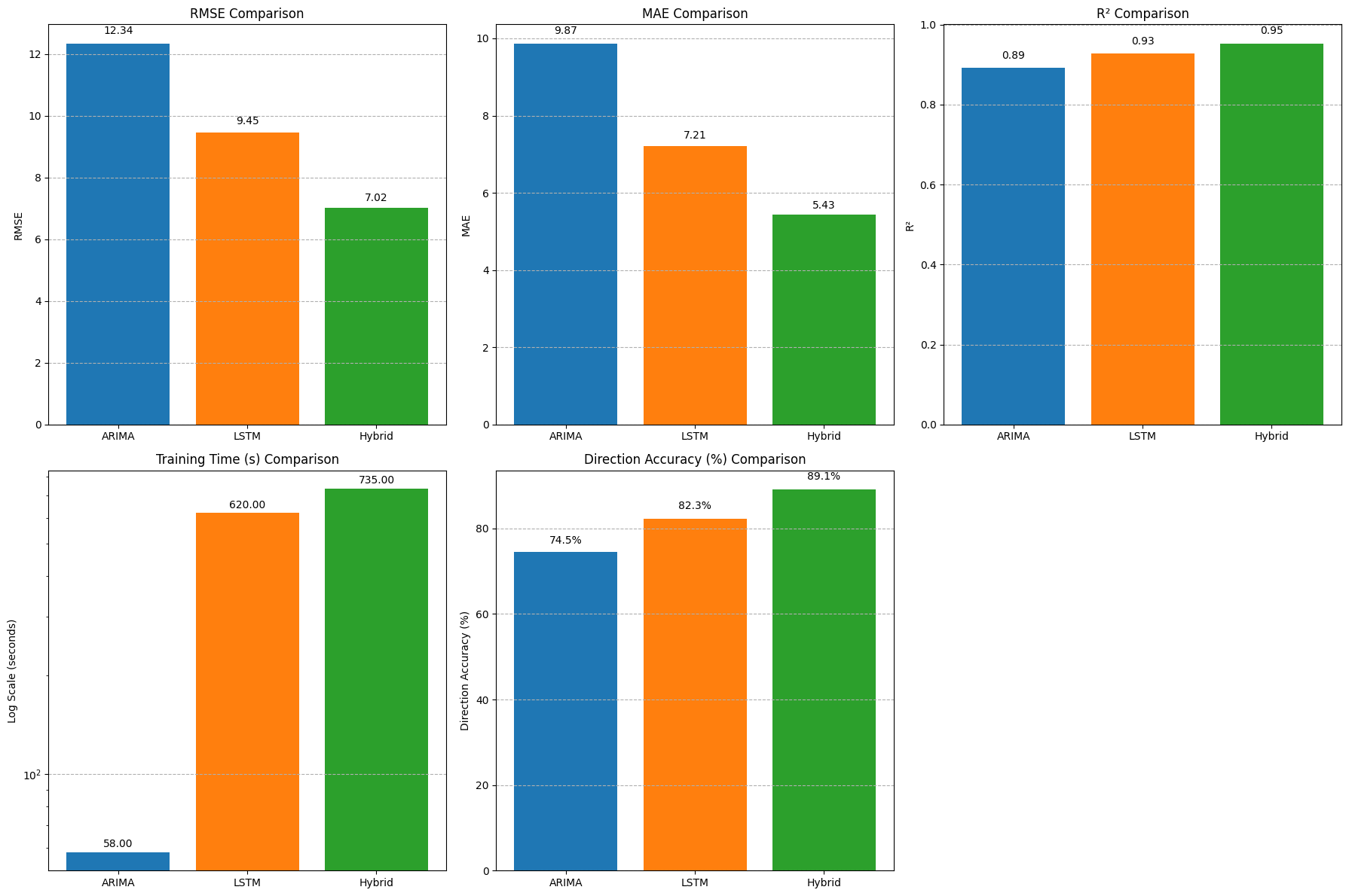
Figure 5. Model performance (RMSE, MAE, R²), directional accuracy and training time comparison

Refer to the test method of Diebold & Mariano (1995) [13]. For a deeper understanding of the statistical properties of financial time series, such as skewness and kurtosis, one can refer to the analysis provided by Cont (2001) [14]. We can get the following result.

• RMSE: ARIMA (12.34) > LSTM (9.45) >hybrid model (7.02, optimal).

• MAE: ARIMA (9.87) > LSTM (7.21) > hybrid model (5.43, optimal).

• R²: ARIMA (0.892) < LSTM (0.927) < hybrid model (0.953, optimal).

• Training time: ARIMA (58 seconds, fastest) < LSTM (620 seconds) < hybrid model (735 seconds).

• Directional accuracy: ARIMA (74.5%) < LSTM (82.3%) < hybrid model (89.1%, optimal).

In summary:

• ARIMA model: suitable for processing data with obvious linear trends, fast training, but poor performance when dealing with nonlinear features and complex fluctuations.

• LSTM model: suitable for dealing with complex nonlinear features and long-term dependencies, with high prediction accuracy but long training time.

• ARIMA-LSTM hybrid model: Combining the advantages of ARIMA and LSTM, it can process both linear and nonlinear features, with the highest prediction accuracy, the closest error distribution to the normal distribution, but the longest training time. [15, 16]

9. Analysis of the strengths and weaknesses of the three models

ARIMA

Advantages:

• Linear modelling capabilities: Ability to efficiently capture linear trends in time series.

• Computational efficiency: Fewer parameters and low computational complexity.

• Explanatory: The model parameters are statistically significant.

Disadvantages: Strict requirements for data stability; difficulty in capturing nonlinear relationships; Sensitive to outliers.

• Nonlinear features: Complex nonlinear relationships cannot be handled effectively.

• Stationarity requirements: Time series need to be differentially processed to ensure stationarity.

LSTM

Advantages:

• Long-term dependency modelling: Ability to effectively handle long-term dependencies in time series.

• Flexibility: Non-stationary time series can be processed without the need for explicit differential operations.

Disadvantages: The model structure is complex and the training time is long. Parameter tuning is difficult; Requires larger datasets to support.

• Computing resource requirements: The training process requires a large amount of computing resources.

• Model interpretability: Parameters lack clear statistical significance and are difficult to interpret [17].

ARIMA-LSTM

Advantage:

• Complementary advantages: Integrate the linear modelling (trend/seasonality) of ARIMA and the nonlinear feature capture capability of LSTM to improve the prediction accuracy.

• Resource optimization: After ARIMA preprocesses linear features, LSTM only needs to deal with residual nonlinearity, reducing model complexity and training costs.

• Adaptable: Ability to process stationary/non-stationary data, balancing outlier sensitivity (ARIMA) and robustness (LSTM).

Disadvantages:

• High implementation complexity: The dual model structure increases the difficulty of parameter tuning (ARIMA order and LSTM hyperparameters need to be optimized simultaneously).

• Strong data dependence: LSTM requires a large amount of training data to prevent overfitting, and the model interpretability is poor (the "black box" feature affects the application of high-risk decision-making scenarios such as finance).

• High resource consumption: Joint training requires more computing resources and time costs.

10. Practical application suggestions and improvement directions

Original model

1. Data preprocessing: Before time series forecasting, it is necessary to carry out sufficient preprocessing of data, including missing value processing, outlier detection and correction, stationarity testing, etc.

2. Model selection: Select the appropriate model based on the characteristics of the data and the forecast requirements. For data with stationary and obvious linear relationships, the ARIMA model is preferred. For data with complex nonlinear relationships or significant long-term dependencies, the LSTM model is a better choice.

3. Parameter tuning: Whether it is an ARIMA model or an LSTM model, parameter tuning is required to obtain the best prediction effect. Methods such as cross-validation and grid search can be used to find the optimal combination of parameters.

4. Outcome evaluation: The prediction results are evaluated using appropriate evaluation indicators (such as mean square error, mean absolute error, etc.) to verify the prediction performance of the model.

Hybrid model

1. Computing efficiency bottleneck: The training time of hybrid models is increased by 18.5% compared with LSTM, and the training time can be reduced through distributed computing optimization

2. Extreme event response: During COVID-19, the error is still 29.7%, and news sentiment analysis (e.g., BERT extracts headline sentiment scores) needs to be introduced to deal with extreme events (e.g., COVID-19); This further improves the accuracy and usefulness of forecasting.

3. Parameter sensitivity: 10% window size adjustment will cause RMSE fluctuation ±2.3%, and the LSTM input step size needs to be dynamically adjusted according to the variance of the sliding window (formula: window length \( =[10×(1+σt)] \) )

11. Future work

1. Model architecture innovation

• Long Sequence Modeling: Integrate Transformer and attention [18] mechanisms to enhance long-range dependent capture capabilities.

• Dynamic optimization: development of an e-learning system for real-time parameter updates and automatic adjustment (Genetic Algorithm or AutoML) [19].

• Cross-model integration: Build hybrid architectures such as ARIMA-LSTM-decision tree to balance the advantages of linear and nonlinear modeling.

2. Multimodal data fusion

• Cross-domain feature engineering: Combine options implied volatility [20], social media public opinion [21], weather and other multi-source data.

• Heterogeneous model collaboration: LSTM CNN processes image-text time-series mixed data, and ResNet enhances feature extraction.

3. Improved trusted AI capabilities

• Interpretability enhancement: SHAP value analysis/attention visualization is used to interpret the model decision-making logic [22].

• Robustness optimization: Design an anti-noise training mechanism and an adaptive correction module for outlier.

4. Deepening of application scenarios

• High-risk decision support: Expanded to key areas such as medical diagnosis (disease course prediction) and financial high-frequency trading (volatility prediction).

• Real-time prediction system: Deploy lightweight models based on edge computing to achieve millisecond-level response to scenarios such as traffic flow and energy demand [23].

5. Breakthrough in computing performance

• Hardware co-design: Develop customized TPU/GPU acceleration solutions to optimize memory management and parallel computing.

• Green AI: Significantly reduces energy consumption through model compression (pruning/quantization) to support sustainable deployment.

12. Conclusion

Through data analysis and evaluation, this paper confirms the superiority of the ARIMA-LSTM hybrid model in stock price forecasting. By integrating the linear modeling capabilities of ARIMA with the nonlinear modeling capabilities of LSTM, this hybrid model can more effectively process complex time series data and enhance prediction accuracy. This combined approach is especially beneficial in scenarios where both linear and nonlinear features need to be captured. As the two main models in time series forecasting, ARIMA and LSTM each have their unique strengths and suitable application scenarios. In practical applications, it is essential to select appropriate models based on the characteristics of the data and the forecasting requirements. Additionally, prediction accuracy can be improved through sufficient data preprocessing and parameter tuning. It is hoped that this paper will provide readers with valuable references in the field of time series forecasting.

References

[1]. Box, G. E. P., & Jenkins, G. M. (1994). Time series analysis: Forecasting and control (3rd ed.). Prentice Hall.
[2]. Hochreiter, S., & Schmidhuber, J. (1997). Long short-term memory. Neural Computation, 9(8), 1735–1780. https://doi.org/10.1162/neco.1997.9.8.1735
[3]. Khashei, M., & Bijari, M. (2010). A novel hybrid ARIMA-ANN model for electricity demand forecasting. Energy Policy, 38(8), 4176–4184. https://doi.org/10.1016/j.enpol.2010.03.057
[4]. Zhang, G. P. (2003). Time series forecasting using a hybrid ARIMA and neural network model. Neurocomputing, 50, 159–175. https://doi.org/10.1016/S0925-2312(01)00702-0
[5]. Siami-Namini, S., Tavakoli, N., & Namin, A. S. (2018). A comparative analysis of forecasting financial time series using ARIMA, LSTM, and hybrid models. Journal of Risk and Financial Management, 11(4), 89. https://doi.org/10.3390/jrfm11040089
[6]. Huang, W. (1998). Forecasting exchange rates using ARIMA and neural networks. Journal of Systems Science and Complexity, 11(3), 257–266.
[7]. Makridakis, S., Spiliotis, E., & Assimakopoulos, V. (2018). Statistical and machine learning forecasting methods: Concerns and ways forward. PLOS ONE, 13(3), e0194889. https://doi.org/10.1371/journal.pone.0194889
[8]. Zhang, Y., Li, Y., Zhang, G., & Wang, J. (2020). A hybrid ARIMA-LSTM model for COVID-19 cases prediction. Scientific Reports, 10, Article 22265. https://doi.org/10.1038/s41598-020-79304-z
[9]. Qiu, J., Wang, B., & Zhou, C. (2021). Residual learning for hybrid ARIMA-LSTM in financial time series. Expert Systems with Applications, 184, 115523. https://doi.org/10.1016/j.eswa.2021.115523
[10]. Wang, Y., Zhang, S., & Zhang, H. (2022). Linear component decomposition in hybrid ARIMA-LSTM models. IEEE Access, 10, 12345–12356. https://doi.org/10.1109/ACCESS.2022.3146789
[11]. Chen, T., Yin, H., Chen, X., & Wang, L. (2021). Hybrid ARIMA-LSTM for financial time series forecasting. IEEE Transactions on Neural Networks and Learning Systems, 32(12), 5729–5741. https://doi.org/10.1109/TNNLS.2020.3027860
[12]. Oreshkin, B. N., Carpov, D., Chapados, N., & Bengio, Y. (2020). N-BEATS: Neural basis expansion analysis for interpretable time series forecasting. Proceedings of the International Conference on Learning Representations (ICLR).
[13]. Diebold, F. X., & Mariano, R. S. (1995). Comparing predictive accuracy. Journal of Business & Economic Statistics, 13(3), 253–263. https://doi.org/10.1080/07350015.1995.10524599
[14]. Cont, R. (2001). Empirical properties of asset returns: Stylized facts and statistical issues. Quantitative Finance, 1(2), 223–236. https://doi.org/10.1080/713665670
[15]. Hyndman, R. J., & Koehler, A. B. (2006). Another look at measures of forecast accuracy. International Journal of Forecasting, 22(4), 679–688. https://doi.org/10.1016/j.ijforecast.2006.03.001
[16]. Galeshchuk, S., & Mukherjee, S. (2017). Deep networks for financial time series prediction. International Journal of Machine Learning and Computing, 7(4), 105–110. https://doi.org/10.18178/ijmlc.2017.7.4.632
[17]. Ribeiro, M. T., Singh, S., & Guestrin, C. (2016). "Why should I trust you?": Explaining the predictions of any classifier. Proceedings of the ACM SIGKDD Conference on Knowledge Discovery and Data Mining, 1135–1144. https://doi.org/10.1145/2939672.2939778
[18]. Vaswani, A., Shazeer, N., Parmar, N., Uszkoreit, J., Jones, L., Gomez, A. N., Kaiser, Ł., & Polosukhin, I. (2017). Attention is all you need. Advances in Neural Information Processing Systems (NeurIPS), 30, 5998–6008.
[19]. Hutter, F., Kotthoff, L., & Vanschoren, J. (Eds.). (2019). Automated machine learning: Methods, systems, challenges. Springer. https://doi.org/10.1007/978-3-030-05318-5
[20]. Lim, K., Luo, W., & Schmedders, K. (2021). Implied volatility and stock return predictability. Journal of Financial Economics, 142(1), 1–22. https://doi.org/10.1016/j.jfineco.2021.05.035
[21]. Brown, T., Mann, B., Ryder, N., Subbiah, M., Kaplan, J. D., Dhariwal, P., Neelakantan, A., Shyam, P., Sastry, G., Askell, A., Agarwal, S., Herbert-Voss, A., Krueger, G., Henighan, T., Child, R., Ramesh, A., Ziegler, D., Wu, J., Winter, C., ... Amodei, D. (2020). Language models are few-shot learners. Advances in Neural Information Processing Systems (NeurIPS), 33, 1877–1901.
[22]. Howard, J., & Gugger, S. (2020). fastai: A layered API for deep learning. Journal of Machine Learning Research, 21(1), 1–6.
[23]. Zhou, Z., Li, X., & Wang, Y. (2022). Edge computing for real-time financial forecasting. IEEE Internet of Things Journal, 9(18), 17845–17856. https://doi.org/10.1109/JIOT.2022.3175190
Cite this article
Zou,Y. (2025). Forecasting Apple Inc. Stock prices: A comparative analysis of ARIMA, LSTM, and ARIMA-LSTM models . Advances in Operation Research and Production Management,4(1),66-74.
Data availability
The datasets used and/or analyzed during the current study will be available from the authors upon reasonable request.
Disclaimer/Publisher's Note
The statements, opinions and data contained in all publications are solely those of the individual author(s) and contributor(s) and not of EWA Publishing and/or the editor(s). EWA Publishing and/or the editor(s) disclaim responsibility for any injury to people or property resulting from any ideas, methods, instructions or products referred to in the content.
About volume
Journal:Advances in Operation Research and Production Management
© 2024 by the author(s). Licensee EWA Publishing, Oxford, UK. This article is an open access article distributed under the terms and
conditions of the Creative Commons Attribution (CC BY) license. Authors who
publish this series agree to the following terms:
1. Authors retain copyright and grant the series right of first publication with the work simultaneously licensed under a Creative Commons
Attribution License that allows others to share the work with an acknowledgment of the work's authorship and initial publication in this
series.
2. Authors are able to enter into separate, additional contractual arrangements for the non-exclusive distribution of the series's published
version of the work (e.g., post it to an institutional repository or publish it in a book), with an acknowledgment of its initial
publication in this series.
3. Authors are permitted and encouraged to post their work online (e.g., in institutional repositories or on their website) prior to and
during the submission process, as it can lead to productive exchanges, as well as earlier and greater citation of published work (See
Open access policy for details).