1. Introduction

Renewal theory is a study of stochastic models where events occur continuously over time, with the intervals between events being independent and identically distributed random variables. Similarly, a renewal process is a recurrent-event process with i.i.d. interarrival times [1]. Renewal theory is a branch of probability that began as the study of probability problems connected with the failure and replacement of components, such as electric light bulbs. Later, it became clear that similar problems also arise in many other applications of probability theory and that the fundamental mathematical theorems of renewal theory are of intrinsic interest in the theory of probability [2].

The purpose of this report is to deepen our understanding of this multi-functional area, focusing on the mathematical constructs that define the renewal process, including the renewal function and the renewal equation, as well as the theorems supporting these constructs.

In the first section of this report, we use a special case of the renewal process - the Poisson process. The Poisson process exhibits all the defining properties of renewal processes and serves as an introductory model for the mathematical foundations and definitions that follow. Several of the methods or definitions will later facilitate proofs within renewal theory. Connections between this section and later definitions, theorems, and examples will be evident throughout the report.

Although we begin with Poisson processes - a stepping stone to understanding more complex renewal processes - we are not limited to their discrete nature. Instead, our exploration extends to continuous models, broadening the analytical perspective. Long-term change is important in renewal processes, as it allows predictions of future behaviour. The report concludes with practical applications that illustrate the relevance and power of renewal theory in modelling real-world systems.

2. Poisson process

Before delving into the Poisson process in detail, we first review some foundational concepts essential for its understanding.

2.1. Exponential and poisson random variables

2.1.1. Exponential random variables

We write  $$ X\sim Exp\left(\lambda \right)$$  if it has density:

$$$ f_X\left(x\right)=\{\begin{array}{c}\lambda e^{-\lambda x}, x\ge 0, \\ 0, x\le 0. \end{array}$$$

Then  $$ E\left[X\right]=1\text{/}\lambda $$   $$ \mathrm{V}\mathrm{a}\mathrm{r}\left(X\right)=1/{\lambda }^2$$ .

Memorylessness property of exponential random variable

Theorem 1. Exponential random variables are memoryless, that is,

$$$ P\left(X>s+tX>s\right)=P\left(X>t\right),\hspace{1em}\forall s,t\ge 0$$$

Proof.

Let  $$ X$$  be an exponential random variable with rate  $$ \lambda $$ . Then the density function of  $$ X$$  is  $$ f_X\left(x\right)=\lambda e^{-\lambda x}$$  . Then,  $$ P\left(X>t\right)={\int }_t^{\text{∞}}{f}_X\left(x\right)dx=e^{-\lambda t}$$ .

$$$ P\left[X>s+tX>s\right]=\frac{P\left(X>s+t\right)}{P\left(X>s\right)}=\frac{e^{-\lambda \left(s+t\right)}}{e^{-\lambda s}}=e^{-\lambda \left(s+t\right)+\lambda s}=e^{-\lambda t}=P\left(X>t\right)\text{.}$$$

Poisson random variables

We write  $$ X\sim \text{Poisson}\left(\lambda \right)$$  if

Moreover,  $$ E\left[X\right]=Var\left(X\right)= \lambda $$ .Proposition 1. The Poisson distribution is additive. Let  $$ X\sim \text{Poisson}\left({\lambda }_1\right)$$  and  $$ Y\sim \text{Poisson}\left({\lambda }_2\right)$$  be independent; then  $$ \left(X+Y\right)\sim \text{Poisson}\left({\lambda }_1+{\lambda }_2\right)$$  .

Proof.

$$$ Pr\left(X+Y=n\right)=e^{-\left({\lambda }_1+{\lambda }_2\right)}\frac{1}{n!}{\sum }_{i=0}^n\left(\frac{n}{i}\right){\lambda }_1^i{\lambda }_2^{n-i}=e^{-\left({\lambda }_1+{\lambda }_2\right)}\frac{{\left({\lambda }_1+{\lambda }_2\right)}^n}{n!}\text{.}$$$

2.2. Counting process

Definition 1 (Counting process). A stochastic process  $$ N\left(t\right),t\ge 0$$  is a counting process if  $$ N\left(t\right)$$  is the total number of events that have occurred by time  $$ t$$[3]. By definition:

 $$ N\left(t\right)\in \mathrm{0,1},2,\dots $$  for all  $$ t\ge 0$$  ;

If  $$ a\le b$$  then  $$ N\left(a\right)\le N\left(b\right)$$  ;

For  $$ a\le b$$  ,  $$ N\left(b\right)-N\left(a\right)$$  equals the number of events in  $$ \left(a,b\right]$$ .

Properties 1. (Counting process) [3]

(i) Independent increments: counts on disjoint intervals are independent.

(ii) Stationary increments: the distribution of  $$ N\left(b\right)-N\left(a\right)$$  depends only on  $$ b-a$$ .

2.3. Definition of poisson process

Definition 2. (Poisson Process) The counting process  $$ N\left(t\right),t\ge 0$$  is said to be a Poisson process with rate  $$ \lambda $$  and  $$ \lambda >0$$  , if:

1.  $$ N\left(0\right)=0$$ , almost surely.

2. The process has independent increments.

3. The number of events in any interval of length  $$ t$$  is Poisson distributed with mean  $$ \lambda t$$  . That is, for all  $$ s,t\ge 0$$  :

$$$ PN\left(t+s\right)-N\left(s\right)=n=e^{-\lambda t}\frac{{\left(\lambda t\right)}^n}{n!},\mathrm{ }n=\mathrm{0,1},$$$

In other words, for  $$ s\le t$$  ,  $$ N\left(t\right)-N\left(s\right)\sim \text{Poisson}\left(\lambda t\right)$$ . We then call  $$ N\left(t\right)$$  a Poisson process with rate  $$ \lambda $$  , such that  $$ E\left[N\left(t\right)\right]=\lambda t$$  .

Verifying conditions (i) and (ii) is straightforward. However, verifying condition (iii) can be challenging. Therefore, we require simpler equivalent conditions to verify "the display in Definition 2 (iii)".

Definition 3. (Definition of o(h)) The function  $$ f$$  is said to be  $$ o\left(h\right)$$  if

$$$ \underset{h\to 0}{lim}\frac{f\left(h\right)}{h}=0.$$$

Changes to the original definition can be made using this function.

Definition 4 [3]. A counting process  $$ N\left(t\right),t\ge 0$$  is said to be a Poisson process having rate  $$ \lambda $$  , and  $$ \lambda >0$$  , if:

(i)  $$ N\left(0\right)=0$$  almost surely.

(ii) The process has stationary and independent increments.

(iii)  $$ PN\left(h\right)=1=\lambda h+o\left(h\right)\text{.}$$ 

(iv)  $$ PN\left(h\right)\ge 2=o\left(h\right)\text{.}$$ 

A full proof of the equivalence appears in [3]

2.4. Interarrival time and waiting time

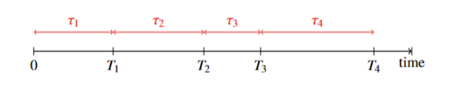
As shown in Figure 1, the simple renewal process illustrates the sequence of interarrival times between successive events.

Let  $$ T_n$$  be the event times of a Poisson process and set  $$ {\tau }_n=T_n-T_{n-1}$$  . For  $$ t\ge 0$$  ,

$$$ Pr\left({\tau }_1>t\right)=Pr\left(N\left(t\right)=0\right)=e^{-\lambda t},$$$

Hence,  $$ {\tau }_1\sim \left\{Exp\right\}\left(\mathrm{\lambda }\right)$$  . By stationary and independent increments, for any  $$ s,t\ge 0$$  ,

$$$ Pr\left({\tau }_2>t{\tau }_1=s\right)=Pr\left(N\left(s+t\right)-N\left(s\right)=0\right)=e^{-\lambda t},$$$

Thus,  $$ {\left({\tau }_n\right)}_{n\ge 1}$$  are i.i.d. { $$ Exp\left\}\right(\lambda )$$ .

Definition 5. The waiting time  $$ S_n={\sum }_{i=1}^n{\tau }_i$$  represents the moment at which the  $$ n$$ -th event occurs.

2.5. Transformation of poisson processes

Let  $$ N_1\left(t\right)$$  and  $$ N_2\left(t\right)$$  be two independent Poisson processes with rates  $$ {\lambda }_1$$  and  $$ {\lambda }_2$$ .

Superposition

Lemma 1.  $$ N\left(t\right)≔N_1\left(t\right)+N_2\left(t\right)$$  is also a Poisson process with rate  $$ {\lambda }_1+{\lambda }_2$$ .

Proof

(i)  $$ N\left(0\right)=0$$  a.s. since  $$ N_1\left(0\right)=N_2\left(0\right)=0$$ .

(ii) Independent increments: for disjoint intervals  $$ I_j$$  the vectors $$ \left(N_1\left(I_j\right),N_2\left(I_j\right)\right) $$ are independent, hence so are  $$ N\left(I_j\right)=N_1\left(I_j\right)+N_2\left(I_j\right)$$ .

(iii) For  $$ s,t\ge 0$$ ,

$$$ N\left(t+s\right)-N\left(s\right)=\left(N_1\left(t+s\right)-N_1\left(s\right)\right)+\left(N_2\left(t+s\right)-N_2\left(s\right)\right),$$$

where the two summands are independent with laws Poisson( $$ {\mathrm{\lambda }}_1$$ 𝑡) and Poisson( $$ {\mathrm{\lambda }}_2$$ 𝑡). By additive proposition, their sum is Poisson (( $$ {\mathrm{\lambda }}_1$$  +  $$ {\mathrm{\lambda }}_2$$ )𝑡). Hence  $$ N$$  is a Poisson process with rate  $$ {\lambda }_1+{\lambda }_2$$ .

Stochastic DominationProposition 2. If  $$ 0<{\lambda }_1\le {\lambda }_2$$  , then  $$ {\left(N_1\left(t\right)\right)}_{t\ge 0}$$  is stochastically dominated by  $$ {\left(N_2\left(t\right)\right)}_{t\ge 0}$$ . In other words,  $$ \exists $$  a coupling of  $$ N_1$$  and  $$ N_2$$  such that  $$ N_1\le N_2$$ . It can be expressed as  $$ N_1\left(t\right)\underset{s}{\le }{N}_2\left(t\right)$$ .

2.6. Compound poisson process

Definition 6 [3]. Let  $$ X_1,X_2,$$  be i.i.d. with cdf  $$ F$$  , and  $$ N\sim \text{Poisson}\left(\lambda \right)$$  independent of  $$ X_1,X_2,$$  . Then we call  $$ W$$ :

$$$ W={\sum }_{i=1}^N{X}_i,$$$

a compound Poisson random variable.

For  $$ W$$ , the expressions for the expected value and variance are provided as follows:

$$$ \begin{array}{cccc}E\left[W\right]& =\lambda E\left[X\right]& \mathrm{ }\mathrm{ }\mathrm{ }\mathrm{ }\mathrm{ }\mathrm{ }\mathrm{ }\mathrm{ }\mathrm{ }\mathrm{ }\mathrm{ }\mathrm{ }\text{Var}\left(W\right)& =\lambda E\left[X^2\right]\end{array}$$$

Remark. For most applications, the first two moments above suffice. The identity  $$ E\left[Wh\left(W\right)\right]=\lambda E\left[Xh\left(W+X\right)\right]$$  (via conditioning on  $$ N$$ ) can generate higher moments when needed, so we omit the proof here.

Definition 7 (Compound Poisson process). Let  $$ N{\left(t\right)}_{t\ge 0}$$  be a Poisson process with rate  $$ \lambda $$  and  $$ X_i$$  i.i.d.\ with cdf  $$ F$$  , independent of  $$ N$$ . Define:

$$$ X\left(t\right)≔{\sum }_{i=1}^{N\left(t\right)}{X}_{i\text{.}}$$$

Then  $$ X\left(t\right)$$  is a compound Poisson process and

$$$ E\left[X\left(t\right)\right]=\lambda tE\left[X\right],\text{Var}\left(X\left(t\right)\right)=\lambda tE\left[X^2\right]\text{.}$$$

This model still enforces exponential interarrivals; to allow arbitrary i.i.d.\ gaps we now consider renewal processes.

3. Renewal process and the elementary renewal theorem

3.1. Renewal process

A renewal process  $$ N=N\left(t\right):t\ge 0$$  is a counting process such that

$$$ N\left(t\right)=\max \mathrm{ }\{n:T_n\le t\},$$$

where  $$ T_0=0$$  and  $$ T_n=X_1+X_2+\dots +X_n$$  for  $$ n\ge 0$$  , and  $$ X_i$$  is a sequence of independent identically distributed non-negative random variables following the distribution  $$ F$$ .

Let the interarrival times  $$ X_i$$  be i.i.d. with cdf  $$ F$$  and mean  $$ \mu $$  , and write  $$ S_n≔T_n={\sum }_{i=1}^n{X}_i$$ . By the strong law of large numbers,

$$$ \frac{S_n}{n}\to \mu \mathrm{ }\left(n\to \text{∞}\right)\text{.}$$$

Hence, for each fixed  $$ t$$ ,  $$ N\left(t\right)=\mathrm{ma}x\mathrm{ }\{n:T_n\le t\}$$  is finite almost surely. A renewal process generalises the Poisson case; exponential interarrivals recover the Poisson process. Figure 2 shows an example of a renewal process.

3.2. Renewal function

Definition 9. The survival function for a random variable  $$ X$$  with distribution  $$ F$$  as  $$ \bar{F}=1-F$$  .

Definition 10. For functions  $$ f,g$$  , their convolution is

$$$ \left(f\mathrm{*}g\right)\left(t\right)={\int }_{-\text{∞}}^{\text{∞}}fg\left(t-\tau \right)d\tau \text{.}$$$

We write  $$ F^{\mathrm{*}n}$$  for the  $$ n$$  -fold convolution of a cdf  $$ F$$  and use  $$ F_n≔F^{\mathrm{*}n}$$  .

Lemma 2. Assume that  $$ F$$  is the distribution function of  $$ X_1$$  , and denote  $$ F_k$$  as the distribution function of  $$ T_k$$ . We have that  $$ F_1=F$$  and  $$ F_{k+1}\left(x\right)={\int }_0^x{F}_k\left(x-y\right)dF\left(y\right) \text{for }k\ge 1.$$ 

When we study the distribution of interarrival time  $$ N\left(t\right)$$ , we will automatically consider its expectation.

Definition 11. Let  $$ M\left(t\right)=E\left[N\left(t\right)\right]\text{.}$$  We call  $$ M\left(t\right)$$  the renewal function.

Proposition 3 [3].

$$$ M\left(t\right)={\sum }_{n=1}^{\text{∞}}{F}_n\left(t\right)\text{.}$$$

Where ( $$ F_n$$ (𝑡) is the n-fold convolution of F.

Proof.

Let  $$ I_{n\mathrm{ }}\{\begin{array}{c} 1 if the nth renewal occurred in [0, t], \\ 0 otherwise.\end{array}$$  Then,  $$ N\left(t\right)={\sum }_{n=1}^{\mathrm{\infty }}{I}_n$$ ,

$$$ E\left[N\left(t\right)\right]=E\left[{\sum }_{n=1}^{\mathrm{\infty }}{I}_n\right]={\sum }_{n=1}^{\mathrm{\infty }}E\left[I_n\right]={\sum }_{n=1}^{\mathrm{\infty }}P\{I_n=1\}={\sum }_{n=1}^{\mathrm{\infty }}P\{S_n\le t\}={\sum }_{n=1}^{\mathrm{\infty }}{F}_n\left(t\right).$$$

Proposition 4.  $$ M\left(t\right)<\mathrm{\infty }\mathrm{ }for\mathrm{ }all\mathrm{ }0\le t<\mathrm{\infty }.$$ 

Truncate interarrivals at a fixed  $$ \alpha >0$$  with  $$ \bar{F}\left(\alpha \right)>0$$ . The truncated process renews only on the grid  $$ n\alpha ,$$  yielding a geometric bound:

$$$ M\left(t\right)\le \frac{\left(t\text{/}\alpha +1\right)}{\bar{F}\left(\alpha \right)}<\text{∞.}$$$

3.3. Elementary renewal theorem

Proposition 5 [3].

$$$ \frac{N\left(t\right)}{t}\to \frac{1}{\mu }\mathrm{ }\text{as}\mathrm{ }\to \text{∞.}$$$

Proof.

We can prove it by using the Squeeze theorem. Firstly, we can find that:

$$$ \frac{S_{N\left(t\right)}}{N\left(t\right)}\le \frac{t}{N\left(t\right)}<\frac{S_{N\left(t\right)+1}}{N\left(t\right)},$$$

since  $$ S_{N\left(t\right)}\le t<S_{N\left(t\right)+1}$$  . We already proved  $$ \frac{S_n}{n}\to \mu \text{as} \to \text{∞}$$ .

Moreover,  $$ \frac{S_{N\left(t\right)+1}}{N\left(t\right)}=\left[\frac{S_{N\left(t\right)+1}}{N\left(t\right)+1}\right]\left[\frac{N\left(t\right)+1}{N\left(t\right)}\right]\text{.}$$  For the same reason above,  $$ \frac{S_{N\left(t\right)+1}}{N\left(t\right)}\to \mu \text{as} \to \text{∞}$$  . Finally, by the Squeeze theorem,  $$ \frac{N\left(t\right)}{t}\to \frac{1}{\mu } \text{as} \to \text{∞.}$$  Thus, we call  $$ \frac{1}{\mu }$$  the rate of the renewal process. In the Poisson process, the rate is typically  $$ \lambda $$  , but not always. Now we may question whether  $$ m\left(t\right)$$  possesses the same convergence.

Stopping Time and Wald’s Equation

Definition 12 [3]. A non-negative integer-valued random variable  $$ N$$  is a stopping time for a sequence  $$ X_1,X_2,$$  if  $$ E\left[N\right]<\text{∞}$$  and  $$ N=n$$  is independent of  $$ X_1,\dots ,X_n$$  .

Theorem 2 [3]. If  $$ X_i$$  are i.i.d. random variables having finite expectations, and if  $$ N$$  is a stopping time for  $$ X_1,X_2,$$  such that  $$ E\left[N\right]<\text{∞}$$ ,

$$$ E\left[{\sum }_{n=1}^N{X}_n\right]=E\left[N\right]E\left[X\right]\text{.}$$$

Proof.

One only needs to construct an indicator function that expresses a finite summation of  $$ X_n$$  as an infinite sum of  $$ E\left[X_n{I}_n\right]$$ .

Corollary 1. If  $$ \mu <\text{∞}$$  then,

$$$ E\left[S_{N\left(t\right)+1}\right]=\mu \left(M\left(t\right)+1\right)\text{.}$$$

The Elementary Renewal Theorem

Theorem 3 [3]. The Elementary Renewal Theorem is:

$$$ \frac{M\left(t\right)}{t}\to \frac{1}{\mu }\mathrm{ }\text{as}\mathrm{ }\to \text{∞.}$$$

Proof.

When  $$ \mu <\text{∞}$$  , we prove the Elementary Renewal Theorem in terms of supremum and infimum.

(Infimum): By the corollary, we can get that  $$ \mu \left(M\left(t\right)+1\right)>t$$  , which implies that:

$$$ \underset{t\to \text{∞}}{\text{liminf}}\frac{M\left(t\right)}{t}\ge \frac{1}{\mu }\text{.}$$$

(Supremum): We cut off the original process, and any interarrival time greater than  $$ Z$$  is truncated to  $$ Z$$ . Then we get a new sequence of interarrival time  $$ \overline{X_i}$$  and new process  $$ \overline{N\left(t\right)}$$  . That is:

$$$ {\bar{X}}_n=\{\begin{array}{cc}{X}_n,& \text{if}{X}_n\le Z,\\ Z,& \text{if}{X}_n>Z\text{.}\end{array}\mathrm{ }n=\mathrm{1,2},\dots $$$

Using Wald's equation,

$$$ {\bar{S}}_{N\left(t\right)+1}\le t+Z⟹\left(\bar{M}\left(t\right)+1\right)E\left[X_n\right]\le t+Z⟹\underset{t\to \text{∞}}{\text{limsup}}\frac{\bar{M}\left(t\right)}{t}\le \frac{1}{E\left[X_n\right]}\text{.}$$$

Since  $$ \overline{S_n}\le S_n$$  , by domination,

$$$ \underset{t\to \text{∞}}{\text{lim sup}}\frac{M\left(t\right)}{t}\le \frac{1}{{\mu }_M}\text{.}$$$

If we let  $$ M\to \text{∞}$$  , we can get

$$$ \underset{t\to \text{∞}}{\text{lim sup}}\frac{M\left(t\right)}{t}\le \frac{1}{\mu }\text{.}$$$

We can do the cut-off again when  $$ \mu =\text{∞}$$  . Since  $$ {\mu }_M\to \text{∞}$$  as  $$ M\to \text{∞}$$  , the answer then becomes obvious from the previous statement.

4. Renewal equation and key renewal theorem

4.1. Renewal equation

Definition 13. When the derivative of  $$ M\left(t\right)$$  exists, its derivative is called the renewal density, denoted as  $$ m\left(t\right)$$ .

Lemma 3. We just need to find the derivative on each side of the equation then,

$$$ m\left(t\right)={\sum }_{n=1}^{\text{∞}}{f}_n\left(t\right)\text{.}$$$

where  $$ f_n$$  is the probability density function of  $$ F_n$$[4].

Lemma 4. Let  $$ M\left(t\right)$$  and  $$ m\left(t\right)$$  respectively satisfy the integral equations:

$$$ M\left(t\right)=F\left(t\right)+{\int }_0^{t}MdF\left(s\right),\mathrm{ }\mathrm{ }\mathrm{ }\mathrm{ }\mathrm{ }\mathrm{ }\mathrm{ }\mathrm{ }\mathrm{ }\mathrm{ }\mathrm{ }\mathrm{ }\mathrm{ }m\left(t\right)=f\left(t\right)+{\int }_0^{t}mds\text{.}$$$

where  $$ f\left(t\right)=F^{\text{'}}\left(t\right)$$ .

Proof.

Write  $$ F_n≔F^{\mathrm{*}n}$$ Since $$ F_n=F_{n-1}\mathrm{*}F$$ we have

$$$ M\left(t\right)={\sum }_{n\ge 1}{F}_n\left(t\right)=F\left(t\right)+{\sum }_{n\ge 2}\left(F_{n-1}\mathrm{*}F\right)\left(t\right)=F\left(t\right)+\left[M\mathrm{*}F\right]\left(t\right),$$$

which yields

$$$ M\left(t\right)=F\left(t\right)+{\int }_0^{t}MdF\left(s\right)\text{.}$$$

When  $$ F$$  has density  $$ f$$  and  $$ M$$  is differentiable, differentiating both sides gives  $$ m\left(t\right)=f\left(t\right)+{\int }_0^{t}mds\text{.}$$ See [1] for details.

Theorem 4. Denote the integral equation of the following form as the renewal equation:

$$$ K\left(t\right)=H\left(t\right)+{\int }_0^{t}KdF\left(s\right)\text{.}$$$

When  $$ t<0$$  ,  $$ H\left(t\right),F\left(t\right)$$  are 0.

Theorem 5. Let  $$ H\left(t\right)$$  in the renewal equation be a bounded function. Then there exists a unique solution to the equation in a finite interval:

$$$ K\left(t\right)=H\left(t\right)+{\int }_0^{t}HdM\left(s\right)\text{.}$$$

Proof.

$$$ K\left(t\right)=H\left(t\right)+\left({\sum }_{n=1}^{\text{∞}}{F}_n\right)\mathrm{*}H\left(t\right)=H\left(t\right)+F\mathrm{*}H\left(t\right)+\left[\left({\sum }_{n=1}^{\text{∞}}{F}_n\mathrm{*}F\right)\mathrm{*}H\left(t\right)\right]$$$

$$$ =H\left(t\right)+F\left[H\left(t\right)+M\mathrm{*}H\left(t\right)\right]=H\left(t\right)+F\mathrm{*}K\left(t\right)=H\left(t\right)+{\int }_0^{t}KdF\left(s\right)\text{.}$$$

Lemma 5 [3].  $$ P\mathrm{ }\{{\mathrm{ }S}_{N\left(t\right)}\le s\mathrm{ }\}=\bar{F}\left(t\right)+{\int }_0^t\bar{F}\left(t-y\right)dM\left(y\right),t\ge s\ge 0.$$ 

4.2. Preparations

Before introducing Blackwell's theorem or the key renewal theorem, it is necessary to distinguish between discrete and continuous cases.

Lattice

Definition 14. A non-negative random variable  $$ X$$  is designated as a lattice if there is a non-negative integer  $$ d$$  such that:

$$ {\sum }_{n=0}^{\text{∞}}P(X=nd)=1$$ .

The maximal value of  $$ d$$  satisfying this condition is referred to as the period of  $$ X$$  .

This property ensures that all the probabilistic mass of  $$ X$$  is concentrated on these discrete points rather than being distributed over a continuous interval. In essence, this indicates that the random variable  $$ X$$  is discrete with periodic properties.

Blackwell's Theorem

Theorem 6 [3]. If  $$ F$$  is non-lattice,

$$$ \underset{t\to \text{∞}}{\mathrm{ }\mathit{lim}m\left(t+a\right)-m\left(t\right)}=\frac{a}{\mu }\mathrm{ }\text{for all }a\ge 0.$$$

If  $$ F$$  is lattice with period  $$ d$$ ,

$$$ \underset{}{\underset{n\to \text{∞}}{\lim }\text{number of renewals at}nd}=\frac{d}{\mu }\text{.}$$$

The full proof of this theorem is lengthy. Detailed proof can be found in [5]. Here, we provide a brief outline.

Brief Proof.

Define $$ g\left(a\right)≔\underset{t\to \mathrm{\infty }}{\lim }\left(m\left(t+a\right)-m\left(t\right)\right)$$  . Additivity gives  $$ g\left(a+x\right)=g\left(x\right)-g\left(a\right)$$  , hence  $$ g\left(a\right)=ca$$  . Let  $$ b_n≔m\left(n\right)-m\left(n-1\right)$$  . Then $$ (\frac{1}{n}{\sum }_{k=1}^n{b}_k=\frac{m\left(n\right)}{n}\underset{n\to \mathrm{\infty }}{\to }1/\mathrm{\mu })$$  by the Elementary Renewal Theorem, so  $$ c=1\text{/}\mu $$  and  $$ g\left(a\right)=a\text{/}\mu $$ .

Put simply, when considering a point in time far from the start of the renewals, the expected number of renewals occurring within a time interval of length 'a' is approximately equal to the length of the interval multiplied by the rate of the renewal process.

Directly Riemann Integration

For any given positive number  $$ a>0$$  , the function  $$ f\left(x\right)$$  is defined on the interval  $$ \left[0,\text{∞}\right)$$  and satisfies:

 $$ {\sum }_{n=1}^{\mathrm{\infty }}\sup \{f\left(x\right):\left(n-1\right)a\le x\le na\}$$ ,  $$ {\sum }_{n=1}^{\mathrm{\infty }}\inf \{f\left(x\right):\left(n-1\right)a\le x\le na\}$$  are finite,

and

 $$ \underset{a\to 0^{+}}{\lim }{\sum }_{n=1}^{\mathrm{\infty }}\sup \{f\left(x\right):\left(n-1\right)a\le x\le na\}$$  = $$ \underset{a\to 0^{+}}{\lim }{\sum }_{n=1}^{\mathrm{\infty }}\inf \{f\left(x\right):\left(n-1\right)a\le x\le na\}$$ 

We say it is directly Riemann Integrable.

4.3. Key renewal theorem

Theorem 7 [3]. When  $$ F$$  is non-lattice and  $$ f\left(t\right)$$  is directly Riemann Integrable, then,

$$$ \underset{t\to \mathrm{\infty }}{\lim }{\int }_0^{t}f\left(t-x\right)\hspace{0.17em}dM\left(x\right)=\frac{1}{\mu }{\int }_0^{\mathrm{\infty }}f\left(t\right)\hspace{0.17em}dt,$$$

where  $$ m\left(x\right)={\sum }_{n=1}^{\text{∞}}{F}_n\left(x\right)\mathrm{ }\text{and}\mathrm{ }\mu ={\int }_0^{\text{∞}}\bar{F}\left(t\right)dt\text{.}$$ 

Proposition 6. The key renewal theorem is equivalent to the Blackwell renewal theorem.

Again, this is a complex proof process and I will only set out some simple proofs.

Short proof.

Assume the Key Renewal Theorem (KRT). For  $$ a>0$$  define  $$ f_a\left(t\right)={\text{1}}_{\left[\text{0,a}\right)}\left(t\right)$$  . Then

$$$ {\int }_0^t{f}_a\left(t-x\right)\hspace{0.17em}dM\left(x\right)\underset{t\to \mathrm{\infty }}{\to }\frac{1}{\mu }{\int }_0^{\mathrm{\infty }}{f}_a\left(u\right)\hspace{0.17em}du=\frac{a}{\mu }.$$$

But

$$$ {\int }_0^t{f}_a\left(t-x\right)\hspace{0.17em}dM\left(x\right)={\int }_{t-a}^{t}1 dM\left(x\right)=M\left(t\right)-M\left(t-a\right)$$$

hence Blackwell’s increment form follows. The converse implication (Blackwell  $$ \Rightarrow $$  KRT) is classical and follows from upper/lower Riemann–sum bounds built from the increments  $$ M\left(t\right)-M\left(t-a\right)$$ ; see [3] or [5].

5. Extension of the renewal process

5.1. Delayed renewal process

Observations often begin mid-cycle (e.g., arriving at a bus stop after the previous bus has departed), so the first interarrival may differ from the rest. In an ordinary renewal process the interarrivals  $$ {\left(X_i\right)}_{i\ge 1}$$  are i.i.d. with cdf  $$ F$$  ; in the delayed case we allow  $$ X_1\sim G$$  while  $$ X_2,X_3,\dots \sim F$$ .

Definition 15 If  $$ X_1$$  follows some other distribution  $$ G$$  and the rest  $$ X_2,X_3,$$  follow the distribution  $$ F$$ , then the counting process  $$ N\left(t\right)$$  is said to be a delayed renewal process, denoted as  $$ N_D\left(t\right)$$ .

Proposition 7. We also denote  $$ M_D\left(t\right)=E\left[N_D\left(t\right)\right], $$ as a delayed renewal function. In the same way as Proposition 3, we can get:

$$$ M\left(t\right)={\sum }_{n=1}^{\text{∞}}G{\mathrm{*}F}_{n-1}\left(t\right)\text{.}$$$

The delayed renewal process has many of the same conclusions as the ordinary renewal process, summarised below.

Proposition 8 [3].

1.By the strong law of large numbers:

$$$ \frac{N_D\left(t\right)}{t}\to \frac{1}{\mu } \text{ as t → ∞.}$$$

2. The Elementary Renewal Theorem for delayed renewal process is also true:

$$$ \frac{M_D\left(t\right)}{t}\to \frac{1}{\mu } \text{as t → ∞.}$$$

3.  $$ M_d\left(t\right)$$  satisfies the integral equations:

$$$ M_d\left(t\right)=F_d\left(t\right)+{\int }_0^t{M}_d\left(t-x\right)dF\left(x\right)\text{.}$$$

4. If  $$ F$$  is non-lattice, it is also satisfied with Blackwell's theorem:

$$$ M_D\left(t+a\right)-M_D\left(t\right)\to \frac{a}{\mu }\mathrm{ }\text{as t → ∞.}$$$

5. If  $$ G$$  and  $$ F$$  are lattice with period  $$ d$$ , then

$$$ \underset{n\text{→ ∞}}{\lim }number\mathrm{ }of\mathrm{ }renewals\mathrm{ }atnd=\frac{d}{\mu }\text{.}$$$

6. The same holds true for the key renewal equations. When  $$ F$$  is non-lattice and  $$ f\left(t\right)$$  is directly Riemann Integrable,

$$$ {\int }_0^{\mathrm{\infty }}f\left(t-x\right)\hspace{0.17em}d{M}_D\left(x\right)\to \frac{1}{\mu }{\int }_0^{\mathrm{\infty }}f\left(t\right)\hspace{0.17em}dt.$$$

Theorem 8 [1]. The process  $$ N^d$$  has stationary increments if and only if

$$$ F^d\left(y\right)=\frac{1}{\mu }{\int }_0^y\left[1-F\left(x\right)\right]\hspace{0.17em}dx$$$

In this case,  $$ M_D\left(t\right)=t\text{/}\mu $$. For complete proof see [2,6].

5.2. Renewal reward process

Renewal models are widespread tools of probability that find application in Queueing Theory, Insurance, Finance, and Statistical Physics among others [6].

Definition 16. Consider the renewal process  $$ N\left(t\right)$$  for interarrival time  $$ X_n,n>0$$  . And it is assumed that each renewal will receive a reward when it occurs. Denote  $$ R_i$$  as the reward received at the  $$ i_{th}$$  renewal and that  $$ R_i$$  is independently and identically distributed. Moreover,  $$ R_i$$  is independent from the  $$ i_{th}$$  interarrival time  $$ X_i$$ . Then we say that  $$ R\left(t\right)$$  is a renewal reward process:

$$$ R\left(t\right)={\sum }_{i=1}^{N\left(t\right)}{R}_{i\text{.}}$$$

It represents the total rewards earned up to time  $$ t$$ .  $$ E\left[R\right]=E\left[R_n\right]$$  ,  $$ E\left[X\right]=E\left[X_n\right]$$  .

Theorem 9 [3]. If  $$ E\left[R\right]<\text{∞}$$  and  $$ E\left[X\right]<\text{∞}$$ , then,

$$$ \frac{R\left(t\right)}{t}\to \frac{E\left[R\right]}{E\left[X\right]}\text{as t → ∞},$$$

$$$ \frac{E\left[R\left(t\right)\right]}{t}\to \frac{E\left[R\right]}{E\left[X\right]}\text{.}$$$

Proof.

Prove (1). When  $$ t\to \text{∞}$$  ,

$$$ \begin{array}{cc}\frac{R\left(t\right)}{t}& =\frac{1}{t}\sum _{i=1}^{N\left(t\right)}{R}_i=\frac{N\left(t\right)}{t}\frac{1}{N\left(t\right)}\sum _{i=1}^{N\left(t\right)}{R}_i=\frac{\frac{\sum _{i=1}^{N\left(t\right)}{R}_i}{N\left(t\right)}}{\frac{t}{N\left(t\right)}}\to \frac{E\left[R\right]}{E\left[X\right]}\text{.}\end{array}$$$

Prove (2). By Wald's equation,  $$ E\left[{\sum }_{i=1}^{N\left(t\right)}{R}_i\right]=E\left[\sum _{i=1}^{N\left(t\right)+1}{R}_i\right]-E\left[R_{N\left(t\right)+1}\right]\approx \left(m\left(t\right)+1\right)E\left[R\right]-E\left[R_{N\left(t\right)+1}\right]\text{.}$$  Multiply both sides of the equation by  $$ \frac{1}{t}$$  ,

$$$ \frac{E\left[R\left(t\right)\right]}{t}=\frac{M\left(t\right)+1}{t}E\left[R\right]-\frac{E\left[R_{N\left(t\right)+1}\right]}{t},$$$

We can get the answer by the elementary renewal theorem if  $$ \frac{E\left[R_{N\left(t\right)+1}\right]}{t}\to 0$$  as  $$ t\to \text{∞}$$ . Since this part of the proof is lengthy, the details can be found in [3].

5.3. Alternating renewal process

Definition 17. In the general renewal process, the system has only one state, e.g. the smoke detector is always on (i.e. it takes no time to change the battery). In real life, replacing the batteries takes time, and the smoke detector belongs to the off state during the time it takes to replace the batteries. We consider that a renewal process with two states, on and off, is called an alternating renewal process.

Remarks:

1.The system alternates between ON periods  $$ Z_1,Z_2,$$  and OFF periods  $$ Y_1,Y_2,$$  ; a renewal occurs at the start of each ON period.

2.The vectors  $$ {\left(Z_n,Y_n\right)}_{n\ge 1}$$  are i.i.d.; hence the cycle lengths  $$ X_n≔Z_n+Y_n$$  are i.i.d.

3.Let  $$ P\left(t\right)=Pr\left(\text{system is ON at time}t\right)$$  and  $$ \overline{P\left(t\right)}=1-P\left(t\right)$$  .

Theorem 10 [3]. If  $$ E\left[Z_n+Y_n\right]<\text{∞}$$  and  $$ F$$  is non-lattice, then

$$$ \underset{t\to \text{∞}}{limP\left(t\right)}=\frac{E\left[Z_n\right]}{E\left[Z_n\right]+E\left[Y_n\right]},$$$

$$$ \underset{t\to \mathrm{\infty }}{\lim }\overline{P\left(t\right)}=\frac{E\left[Y_n\right]}{E\left[Z_n\right]+E\left[Y_n\right]}.$$$

Proof.

Consider a renewal rewards process. Assume that the reward is one per time unit while the system is ON. Also, we don't get any rewards when the system is OFF. So the total reward up to time  $$ t$$  is equal to the total time in which the system is ON in time  $$ \left(0,t\right)$$ . Thus,

$$$ \begin{array}{cc}\underset{t\to \text{∞}}{limP\left(t\right)}& =\underset{t\to \text{∞}}{lim\frac{\text{total ON time in}\left[0,t\right]}{t}}\\ & =\underset{t\to \text{∞}}{lim\frac{R\left(t\right)}{t}}\\ & =\frac{E\left[R\right]}{E\left[X\right]}=\frac{E\left[Z\right]}{E\left[X\right]}=\frac{E\left[Z\right]}{E\left[Z\right]+E\left[Y\right]}\text{.}\end{array}$$$

5.4. Age dependent branching processes

We are interested in self-renewing and growing populations where the ages of current members are easily available and growth can be modelled as a branching process [7]. We consider an organism that can split itself and reproduce. They will produce  $$ j$$  offspring at death by probability  $$ P_j$$  . Each individual's survival time is independently and identically distributed and follows the distribution  $$ F$$ . And so this organism continues to split.

Definition 18 [3]. Denote  $$ X\left(t\right)$$  as the number of individuals in this population of organisms at the time  $$ t$$  .  $$ X\left(t\right),t\ge 0$$  makes up a stochastic process that we call an age-dependent branching process.

Remark. We let  $$ M\left(t\right)=E\left[X\left(t\right)\right]$$  , and  $$ m={\sum }_{j=0}^{\text{∞}}j{P}_j>1$$  , otherwise, it's hard to keep this population alive. For  $$ M\left(t\right)$$  there is the following conclusion:

Theorem 11 [3]. If  $$ F$$  is non-lattice, then:

$$$ \underset{t\to \text{∞}}{lim}{e}^{-\alpha t}M\left(t\right)=\frac{m-1}{m^2\alpha {\int }_0^{\text{∞}}x{e}^{-\alpha x}dF\left(x\right)},$$$

where  $$ \alpha $$  is the only positive number that makes  $$ {\int }_0^{\text{∞}}{e}^{-\alpha x}dF\left(x\right)=\frac{1}{m}\text{.}$$ 

Short proof.

Condition on the lifetime  $$ T_1$$  of the initial individual. Then:

$$$ M\left(t\right)=\bar{F}\left(t\right)+m{\int }_0^{t}Md\bar{F}\left(s\right)\text{.}$$$

Let  $$ \alpha >0$$  be the unique solution of  $$ {\int }_0^{\text{∞}}{e}^{-\alpha x}dF\left(x\right)=1\text{/}m$$  and define

$$$ G\left(s\right)=m{\int }_0^s{e}^{-\alpha y}dF\left(y\right)\text{.}$$$

Set  $$ f\left(t\right)≔e^{-\alpha t}M\left(t\right)$$ ,  $$ h\left(t\right)≔e^{-\alpha t\bar{F}}\left(t\right)$$  Multiplying the previous renewal equation by  $$ e^{-\alpha t}$$  yields

$$$ f\left(t\right)=h\left(t\right)+{\int }_0^{t}fdG\left(s\right)\text{.}$$$

By the Key Renewal Theorem,

$$$ \underset{t\to \text{∞}}{\lim }f\left(t\right)=\frac{{\int }_0^{\text{∞}}hdu}{{\int }_0^{\text{∞}}xdG\left(x\right)}\text{.}$$$

Compute

$$$ {\int }_0^{\text{∞}}h\left(u\right)du={\int }_0^{\text{∞}}{e}^{-\alpha u\bar{F}}\left(u\right)du=\frac{1}{\alpha }\left(1-\frac{1}{m}\right),\mathrm{ }\mathrm{ }\mathrm{ }\mathrm{ }\mathrm{ }\mathrm{ }\mathrm{ }\mathrm{ }\mathrm{ }\mathrm{ }\mathrm{ }\mathrm{ }\mathrm{ }\mathrm{ }\mathrm{ }\mathrm{ }{\int }_0^{\text{∞}}xdG\left(x\right)=m{\int }_0^{\text{∞}}x{e}^{-\alpha x}dF\left(x\right)\text{.}$$$

Therefore,

$$$ \underset{t\to \text{∞}}{lim}{e}^{-\alpha t}M\left(t\right)=\frac{m-1}{m^2\alpha {\int }_0^{\text{∞}}x{e}^{-\alpha x}dF\left(x\right)}\text{.}$$$

6. Some applications

Renewal theory plays an important role in our lives. In this section, we consider some applications of the renewal theory. Due to space constraints, some computations are omitted. Some shorter examples will be fully presented.

6.1. Application of renewal equations in demography

Example 1. Let  $$ B\left(t\right)$$  denote the birth rate at time  $$ t$$  so  $$ B\left(t\right)dt$$  births occur in  $$ \left[t,t+dt\right]$$  ),  $$ S\left(x\right)$$  the survival probability to age  $$ x$$  , and  $$ \beta \left(x\right)$$  the age-specific birth intensity. Then

$$$ B\left(t\right)={\int }_0^{\text{∞}}B(t-x)S\left(x\right)\beta \left(x\right)dx\text{.}$$$

Write  $$ f\left(x\right)=S\left(x\right)\beta \left(x\right)$$  and  $$ F\left(x\right)={\int }_0^{x}f\left(u\right)du$$ ; thus  $$ F\left(\text{∞}\right)$$  is the lifetime expected number of births.

If  $$ F\left(\text{∞}\right)>1$$  , one obtains  $$ B\left(t\right)\sim C{e}^{-Rt} \left(t\to \text{∞}\right),$$  for some constant  $$ C>0$$  , where  $$ R$$  satisfies

$$$ {\int }_0^{\text{∞}}{e}^{Ry}S\left(y\right)\beta \left(y\right)dy=1.$$$

If  $$ F\left(\text{∞}\right)=1$$  , the birth rate converges to a finite positive level; if  $$ F\left(\text{∞}\right)<1$$  , then  $$ B\left(t\right)\to 0$$  exponentially.

References

[1]. Grimmett, G.R., & Stirzaker, D.R. (1992). Probability and Random Processes (Third Edition). Oxford University Press, New York, NY.
[2]. D. R. Cox. (1962). Renewal Theory. Methuen Ltd., London.
[3]. Ross, S.M. Stochastic Processes (Second Editions). Wiley.
[4]. Pinsky, M.A., & Karlin, S. (2011). An Introduction to Stochastic Modeling (Fourth Edition). Academic Press.
[5]. Lindvall, T. (1977). A probabilistic proof of Blackwell’s renewal theorem.Ann. Probab., 5(3), 482-485.
[6]. Zamparo, M. (2023). Large deviation principles for renewal–reward processes. Stoch. Proc. Appl., 156, 226–245.
[7]. Johnson, R.A., & Taylor, J.R. (2008). Preservation of some life length classes for age distributions associated with age-dependent branching processes.Stat. Probab. Lett., 78(17), 2981–2987.
Cite this article
Xie,Y. (2025). Renewal theory. Advances in Operation Research and Production Management,4(3),53-67.
Data availability
The datasets used and/or analyzed during the current study will be available from the authors upon reasonable request.
Disclaimer/Publisher's Note
The statements, opinions and data contained in all publications are solely those of the individual author(s) and contributor(s) and not of EWA Publishing and/or the editor(s). EWA Publishing and/or the editor(s) disclaim responsibility for any injury to people or property resulting from any ideas, methods, instructions or products referred to in the content.
About volume
Journal:Advances in Operation Research and Production Management
© 2024 by the author(s). Licensee EWA Publishing, Oxford, UK. This article is an open access article distributed under the terms and
conditions of the Creative Commons Attribution (CC BY) license. Authors who
publish this series agree to the following terms:
1. Authors retain copyright and grant the series right of first publication with the work simultaneously licensed under a Creative Commons
Attribution License that allows others to share the work with an acknowledgment of the work's authorship and initial publication in this
series.
2. Authors are able to enter into separate, additional contractual arrangements for the non-exclusive distribution of the series's published
version of the work (e.g., post it to an institutional repository or publish it in a book), with an acknowledgment of its initial
publication in this series.
3. Authors are permitted and encouraged to post their work online (e.g., in institutional repositories or on their website) prior to and
during the submission process, as it can lead to productive exchanges, as well as earlier and greater citation of published work (See
Open access policy for details).